External Forcing Conditions#
Up next, we will generate the external forcing conditions that will be used in the California regional model.
First, import packages to re-create and visualize the model fields here:
import os
import numpy as np
from scipy.interpolate import griddata
import matplotlib.pyplot as plt
from matplotlib.gridspec import GridSpec
import netCDF4 as nc4
import cmocean.cm as cm
Next, define the location of the input directory for the model. This is the same directory that holds the bathymetry file and the initial conditions file generated in the previous notebooks for this model example.
# define the input directory
input_dir = '../data/input'
External Forcing Source Files#
For this example, I will use the external forcing fields from the ECCO Version 5 state estimate. I will prepare these fields in 5 steps:
download 7 external forcing fields used in the ECCO model
read the external forcing fields used in the ECCO model as well as the ECCO grid
read in the bathymetry for my model as well as its grid
interpolate the ECCO fields onto my model grid and store each as a binary file
plot the interpolated fields to ensure they look as expected
Step 1: Download the ECCO external forcing fields#
To begin, download the ECCO external forcing fields used in the ECCO Version 5 Alpha state estimate. These fields are available HERE. For my model, I donwloaded the following list of files for my year of interest (2008):
Variable |
File Name |
|---|---|
ATEMP |
EIG_tmp2m_degC_plus_ECCO_v4r1_ctrl |
AQH |
EIG_spfh2m_plus_ECCO_v4r1_ctrl |
SWDOWN |
EIG_dsw_plus_ECCO_v4r1_ctrl |
LWDOWN |
EIG_dlw_plus_ECCO_v4r1_ctrl |
UWIND |
EIG_u10m |
VWIND |
EIG_v10m |
PRECIP |
EIG_rain_plus_ECCO_v4r1_ctrl |
Define the location where these grids are stored:
data_folder = '../data/ECCO'
Step 2: Read in the external forcing fields#
To read in the ECCO fields, I will rely on the exf module from the eccoseas package. I import them here:
from eccoseas.ecco import exf
Next, I will loop through all of the files I downloaded, reading them in with the exf module.
# make a file dictionary to loop over
file_prefix_dict = {'ATEMP':'EIG_tmp2m_degC_plus_ECCO_v4r1_ctrl',
                    'AQH':'EIG_spfh2m_plus_ECCO_v4r1_ctrl',
                    'SWDOWN':'EIG_dsw_plus_ECCO_v4r1_ctrl',
                    'LWDOWN':'EIG_dlw_plus_ECCO_v4r1_ctrl',
                    'UWIND':'EIG_u10m',
                    'VWIND':'EIG_v10m',
                    'PRECIP':'EIG_rain_plus_ECCO_v4r1_ctrl'}

variable_names = list(file_prefix_dict.keys())
# make a list to hold all of the exf grid
exf_grids = []
year=2008

# loop through each variable to read in the grid
for field in variable_names:
    exf_lon, exf_lat, exf_grid = exf.read_ecco_exf_file(data_folder, file_prefix_dict[field], year)
    exf_grids.append(exf_grid)
With an eye toward the interpolation that will come in step 4, I will make 2D grids of longitudes and latitudes to use in the interpolation
Exf_Lon, Exf_Lat = np.meshgrid(exf_lon, exf_lat)
ecco_points = np.column_stack([Exf_Lon.ravel(), Exf_Lat.ravel()])
In addition, I will make a mask to determine where the interpolation will take place. Since the external forcing conditions are provided everywhere, I just set the entire grid to 1:
ecco_mask = np.ones((np.size(Exf_Lon),))
Step 3: Read in the Model Grid#
Next, I will recreate the grid I will use in my model and read in the bathymetry file (see previous notebooks for details):
# define the parameters that will be used in the data file
delX = 1/12
delY = 1/16
xgOrigin = -135
ygOrigin = 29
n_rows = 360
n_cols = 240

# recreate the grids that will be used in the model
xc = np.arange(xgOrigin+delX/2, xgOrigin+n_cols*delX, delX)
yc = np.arange(ygOrigin+delY/2, ygOrigin+n_rows*delY+delY/2, delY)
XC, YC = np.meshgrid(xc, yc)

# read in the bathymetry file
bathy = np.fromfile(os.path.join(input_dir,'CA_bathymetry.bin'),'>f4').reshape(np.shape(XC))
Similar to above, I will make a mask to determine where the interpolatation will take place. I will create this mask using the hFac module from the eccoseas package:
from eccoseas.downscale import hFac
surface_mask = hFac.create_surface_hFacC_grid(bathy, delR=1)
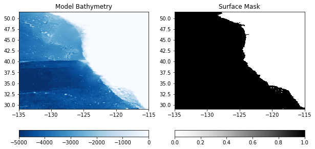
To double check the mask was created as expected, I will plot it in comparison to the bathymetry here:
plt.figure(figsize=(10,5))

plt.subplot(1,2,1)
C = plt.pcolormesh(XC, YC, bathy, vmin=-5000, vmax=0, cmap='Blues_r')
plt.colorbar(C, orientation = 'horizontal')
plt.title('Model Bathymetry')

plt.subplot(1,2,2)
C = plt.pcolormesh(XC, YC, surface_mask, vmin=0, vmax=1, cmap='Greys')
plt.colorbar(C, orientation = 'horizontal')
plt.title('Surface Mask')

plt.show()
Step 4: Interpolate the Fields onto the Model Grid#
Next, I will interpolate the ECCO external fields I read in onto my model domain. I will use the horizonal module from the eccoseas package to accomplish this interpolation.
from eccoseas.downscale import horizontal
❗ Warning#
This code block may take a while to run. Further, it will generate 7 files sized ~500MB. Plan accordingly.
# ensure the output folder exists
if 'exf' not in os.listdir(input_dir):
    os.mkdir(os.path.join(input_dir, 'exf'))
# number of timesteps
n_timesteps = 1
# n_timesteps = np.shape(exf_grid)[0]): # uncomment after testing

# loop through each variable and corresponding ECCO grid
for variable_name, exf_grid in zip(variable_names, exf_grids):

    # print a message to keep track of which variable we are working on
    # uncomment to use
    print('    - Interpolating the '+variable_name+' grid')

    # create a grid of zeros to fill in
    interpolated_grid = np.zeros((np.shape(exf_grid)[0], np.shape(XC)[0], np.shape(XC)[1]))

    # loop through each timestep to generate the interpolated grid
    for timestep in range(n_timesteps):

        # print a message every 100 timesteps to show where we are in the stack
        # uncomment to use
        if timestep%100==0:
            print('        - Working on timestep '+str(timestep)+' of '+str(np.shape(interpolated_grid)[0]))

        # grab the values for this timestep and run the interpolation function
        ecco_values = exf_grid[timestep, :, :].ravel()
        interp_timestep = horizontal.downscale_2D_points_with_zeros(ecco_points, ecco_values, ecco_mask,
                                                                    XC, YC, surface_mask)
        interpolated_grid[timestep,:,:] = interp_timestep

    # convert ECCO values to MITgcm defaults
    if variable_name=='ATEMP':
        interpolated_grid += 273.15
    if variable_name in ['SWDOWN','LWDOWN']:
        interpolated_grid *=-1

    # output the interpolated grid
    output_file = os.path.join(input_dir,'exf',variable_name+'_'+str(year))
    interpolated_grid.ravel('C').astype('>f4').tofile(output_file)
    - Interpolating the ATEMP grid
        - Working on timestep 0 of 1464
    - Interpolating the AQH grid
        - Working on timestep 0 of 1464
    - Interpolating the SWDOWN grid
        - Working on timestep 0 of 1464
    - Interpolating the LWDOWN grid
        - Working on timestep 0 of 1464
    - Interpolating the UWIND grid
        - Working on timestep 0 of 1464
    - Interpolating the VWIND grid
        - Working on timestep 0 of 1464
    - Interpolating the PRECIP grid
        - Working on timestep 0 of 1464
Step 5: Plotting the External Forcing Fields#
Now that the fields have been generated, I will plot them to ensure they look as expected. First, I’ll generate some metadata for each one:
meta_dict = {'ATEMP':[273, 290, cm.thermal, '$^{\circ}$C'],
             'AQH':[0, 0.025, cm.tempo, 'kg/kg'],
             'PRECIP':[0, 1e-6, cm.tempo, 'm/s'],
             'SWDOWN':[-10,20,cm.solar,'W/m$^2$'],
             'LWDOWN':[-100, 500,cm.solar,'W/m$^2$'],
             'UWIND':[-20, 20, cm.balance, 'm/s'],
             'VWIND':[-20, 20, cm.balance, 'm/s'],
             'RUNOFF':[0, 2e-8, cm.tempo, 'm/s']}
Then, I’ll create all of the subplots:
fig = plt.figure(figsize=(8,10))
gs = GridSpec(4, 2, wspace=0.4, hspace=0.03,
              left=0.11, right=0.9, top=0.95, bottom=0.05)


for i in range(len(variable_names)):
    variable_name = variable_names[i]

    CA_exf_grid = np.fromfile(os.path.join(input_dir,'exf',variable_name+'_'+str(year)),'>f4')
    CA_exf_grid = CA_exf_grid.reshape((np.shape(exf_grid)[0],np.shape(XC)[0], np.shape(XC)[1]))

    # choose just the first timestep for plotting
    CA_exf_grid = CA_exf_grid[0, :, :]

    ax1 = fig.add_subplot(gs[i])
    C = plt.pcolormesh(XC, YC, CA_exf_grid,
                       vmin=meta_dict[variable_names[i]][0],
                       vmax=meta_dict[variable_names[i]][1],
                       cmap=meta_dict[variable_names[i]][2])
    plt.colorbar(C, label=variable_names[i]+' ('+meta_dict[variable_names[i]][3]+')',fraction=0.026)

    if i<5:
        plt.gca().set_xticklabels([])
    else:
        plt.gca().set_xlabel('Longitude')
    if i%2==1:
        plt.gca().set_yticklabels([])
    if i==7:
        plt.gca().axis('off')
    if i==2:
        plt.gca().set_ylabel('Latitude')

plt.show()
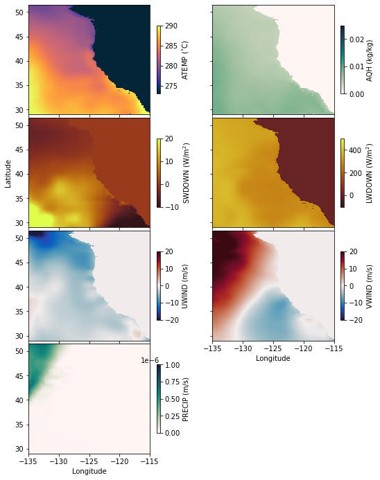
Looks good! Only one more step and then we’re ready to run the model.