Defining the Model Grid#
The model grid for a simulation needs to be configured at both compile time and run time. There are two main options for configuring grids – regular grids and more complex grids using the exch2 package.
Rectangular Grids#
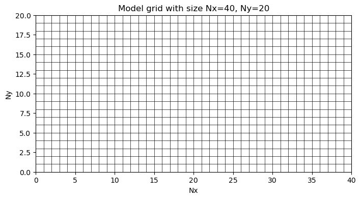
Consider a simple ocean model domain that has dimensions of 40 cells in the x-direction (Nx), 20 cells in the y-direction (Ny), and 10 cells in the z-direction (Nr). In python ordering, this grid has dimensions (10, 20, 40):
import numpy as np
Nx = 40
Ny = 20
Nr = 10
grid = np.zeros((Nr, Ny, Nx))
print('Grid shape:',np.shape(grid))
Grid shape: (10, 20, 40)
We could visualize this grid in the horizontal direction as follows:
import matplotlib.pyplot as plt

# define the cell edges
x_cell_edges = np.arange(Nx+1)
y_cell_edges = np.arange(Ny+1)

# plot the grid
fig = plt.figure(figsize = (8,4))
for i in range(Nx+1):
    plt.plot(x_cell_edges[i]*np.ones((Ny+1,)), y_cell_edges, 'k-', linewidth=0.5)
for j in range(Ny+1):
    plt.plot(x_cell_edges, y_cell_edges[j]*np.ones((Nx+1,)), 'k-', linewidth=0.5)

# format and show
plt.gca().set_xlim([0,Nx])
plt.gca().set_ylim([0,Ny])
plt.xlabel('Nx')
plt.ylabel('Ny')
plt.title('Model grid with size Nx='+str(Nx)+', Ny='+str(Ny))
plt.show()
Compile time files for regular grids#
The key compile time file for generating the model grid is the SIZE.h file. A custom SIZE.h file must be created for each model configuration otherwise the model will not compile.
In the SIZE.h file, Nr is specified directly. However, Nx and Ny are a function of how the grid is partitioned for parallelization. If the model is only going to be run on one CPU, then set sNx = Nx and sNy = Ny in the SIZE.h file.
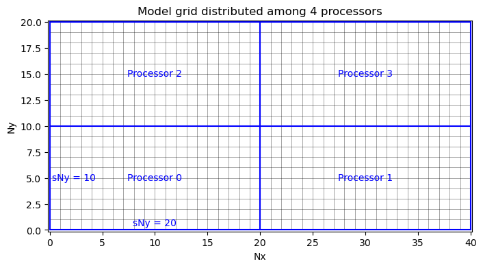
When partitioning the grid to be run in parallel, the domain is divided into tiles of size (sNy, sNy) where sNy is the number of rows in the processing tile and sNx is the number of columns. Each tile will be run on a separate CPU with Px total processors in the x-direction and Py total processeors in the y-direction for a total number of processors Px*Py.
For example, we could define our processing tiles to have size sNx=20 and sNy=10, so that Px=2 and Py=2, visualized as follows:
fig = plt.figure(figsize = (8,4))

# plot the main grid
for i in range(Nx+1):
    plt.plot(x_cell_edges[i]*np.ones((Ny+1,)), y_cell_edges, 'k-', linewidth=0.5, alpha = 0.5)
for j in range(Ny+1):
    plt.plot(x_cell_edges, y_cell_edges[j]*np.ones((Nx+1,)), 'k-', linewidth=0.5, alpha = 0.5)

# plot each processor
sNx = 20
sNy = 10
plt.plot(x_cell_edges[0]*np.ones((Ny+1,)), y_cell_edges, 'b-')
plt.plot(x_cell_edges[sNx]*np.ones((Ny+1,)), y_cell_edges, 'b-')
plt.plot(x_cell_edges[-1]*np.ones((Ny+1,)), y_cell_edges, 'b-')
plt.plot(x_cell_edges, y_cell_edges[0]*np.ones((Nx+1,)),'b-')
plt.plot(x_cell_edges, y_cell_edges[sNy]*np.ones((Nx+1,)),'b-')
plt.plot(x_cell_edges, y_cell_edges[-1]*np.ones((Nx+1,)),'b-')

# annotate
plt.text(sNx/2,sNy/2,'Processor 0', color='blue', ha='center',va='center')
plt.text(sNx*1.5,sNy/2,'Processor 1', color='blue', ha='center',va='center')
plt.text(sNx/2,sNy*1.5,'Processor 2', color='blue', ha='center',va='center')
plt.text(sNx*1.5,sNy*1.5,'Processor 3', color='blue', ha='center',va='center')
plt.text(0.2,sNy/2,'sNy = '+str(sNy), color='blue', ha='left',va='center')
plt.text(sNx/2,0.2,'sNy = '+str(sNx), color='blue', ha='center',va='bottom')

# format and show
plt.gca().set_xlim([-0.15,Nx+0.15])
plt.gca().set_ylim([-0.15,Ny+0.15])
plt.xlabel('Nx')
plt.ylabel('Ny')
plt.title('Model grid distributed among 4 processors')
plt.show()
There is also an option for multi-threading, which is similar to the case for multiprocessing, However, this is not commonly used on computing clusters, so a full description is omitted here.
Runtime files for regular grids#
There are several options for generating a regular model grid. Most options are specified in the data file in the PARM04 namelist.
Specifying grid in the data file#
When using a simple evenly-spaced grid, the grid can be specified directly in the PARM04 namelist. For example, consider the regular grid above with a 20 km spacing in both the x- and y- directions. This would be specified in the PARM04 namelist as:
usingCartesianGrid=.TRUE.,
delX=40*20.E3,
delY=20*20.E3,
xgOrigin= 0.E3,
ygOrigin= 0.E3,
Specifying grids in a tile file#
There is also an option to store your grids in a “tile file” to have them read at run time. When no grid information is provided in the data file and the option usingCurvilinearGrid is specified in PARM04, the model will search for the tile file in the run directory at run time. For model run on a sinple CPU, the file should be named tile001.mitgrid. When running on multple CPUs, the tile files are specific to each processing tile and the names are incremented, e,g. tile001.mitgrid, tile002.mitgrid, tile003.mitgrid, and tile004.mitgrid.
Note
When using multiple processors, a separate tile file must be provided for each processing tile.
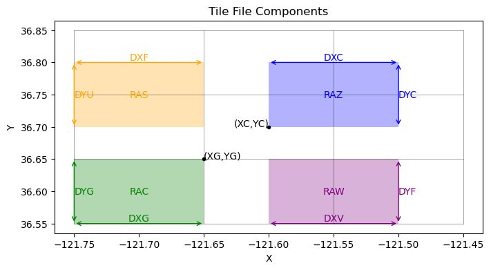
A tile file is composed of 16 different fields organized in a stack of size (16, Ny, Nx) where the 16 fields are defined as follows:
Variable Name |
Description |
|---|---|
XC |
X-coordinate of cell center |
YC |
Y-coordinate of cell center |
DXF |
Cell width measured between cell edges on the top of the cell |
DYF |
Cell height measured between cell edges on the right side of the cell |
RAC |
Cell area measured in rectangle centered in the center of the cells |
XG |
X-coordinate of cell lower-left corner |
YG |
Y-coordinate of cell lower-left corner |
DXV |
Cell width measured between cell centers on the bottom of the cell |
DYU |
Cell height measured between cell centers on the left side of the cell |
RAZ |
Cell area measured in rectangle centered on the corners of the cells |
DXC |
Cell width measured between cell center points |
DYC |
Cell height measured between cell center points |
RAW |
Cell area measured in rectangle centered on the left side of the cells |
RAS |
Cell area measured in rectangle centered on the bottom side of the cells |
DXG |
Cell width measured between lower-left corner points |
DYG |
Cell height measured between lower-left corner points |
If you would like to create a tile file manually, it’s highly recommended that you check out the simplegid package designed to generate these these fields when provided with XC and YC.
We can visualize these fields as follows:
from matplotlib.patches import Rectangle

fig = plt.figure(figsize = (8,4))

# define the grid
xg = np.arange(-121.75,-121.36,0.1)
yg = np.arange(36.55,36.94,0.1)
XG, YG = np.meshgrid(xg, yg)
xc = np.arange(-121.7,-121.49,0.1)
yc = np.arange(36.6,36.9,0.1)
XC, YC = np.meshgrid(xc, yc)

# plot the grid
for i in range(len(xg)):
    plt.plot(xg[i]*np.ones((len(yg),)), yg, 'k-', linewidth=0.5, alpha = 0.5)
for j in range(len(yg)):
    plt.plot(xg, yg[j]*np.ones((len(xg),)), 'k-', linewidth=0.5, alpha = 0.5)
# plt.plot(XC,YC,'k.')
# plt.plot(XG,YG,'k.')

# annotate
plt.text(xc[1],yc[1],'(XC,YC)', ha='right')
plt.text(xg[1],yg[1],'(XG,YG)')
plt.plot(xc[1],yc[1],'k.')
plt.plot(xg[1],yg[1],'k.')

plt.annotate('', xy=(xc[1],yc[2]), xytext=(xc[2],yc[2]), arrowprops=dict(arrowstyle='<->', color='blue'))
plt.text(xg[2],yc[2],'DXC',color='blue',ha='center',va='bottom')
plt.annotate('', xy=(xc[2],yc[1]), xytext=(xc[2],yc[2]), arrowprops=dict(arrowstyle='<->', color='blue'))
plt.text(xc[2],yg[2],'DYC',color='blue',ha='left',va='center')
plt.gca().add_patch(Rectangle((xc[1],yc[1]), xc[2]-xc[1], yc[2]-yc[1],
                              facecolor='blue', alpha=0.3))
plt.text(xg[2],yg[2],'RAZ',color='blue',ha='center',va='center')

plt.annotate('', xy=(xg[0],yc[2]), xytext=(xg[1],yc[2]), arrowprops=dict(arrowstyle='<->', color='orange'))
plt.text(xc[0],yc[2],'DXF',color='orange',ha='center',va='bottom')
plt.annotate('', xy=(xg[0],yc[1]), xytext=(xg[0],yc[2]), arrowprops=dict(arrowstyle='<->', color='orange'))
plt.text(xg[0],yg[2],'DYU',color='orange',ha='left',va='center')
plt.gca().add_patch(Rectangle((xg[0],yc[1]), xg[2]-xg[1], yc[2]-yc[1],
                              facecolor='orange', alpha=0.3))
plt.text(xc[0],yg[2],'RAS',color='orange',ha='center',va='center')

plt.annotate('', xy=(xg[0],yg[0]), xytext=(xg[1],yg[0]), arrowprops=dict(arrowstyle='<->', color='green'))
plt.text(xc[0],yg[0],'DXG',color='green',ha='center',va='bottom')
plt.annotate('', xy=(xg[0],yg[0]), xytext=(xg[0],yg[1]), arrowprops=dict(arrowstyle='<->', color='green'))
plt.text(xg[0],yc[0],'DYG',color='green',ha='left',va='center')
plt.gca().add_patch(Rectangle((xg[0],yg[0]), xg[1]-xg[0], yg[1]-yg[0],
                              facecolor='green', alpha=0.3))
plt.text(xc[0],yc[0],'RAC',color='green',ha='center',va='center')

plt.annotate('', xy=(xc[1],yg[0]), xytext=(xc[2],yg[0]), arrowprops=dict(arrowstyle='<->', color='purple'))
plt.text(xg[2],yg[0],'DXV',color='purple',ha='center',va='bottom')
plt.annotate('', xy=(xc[2],yg[0]), xytext=(xc[2],yg[1]), arrowprops=dict(arrowstyle='<->', color='purple'))
plt.text(xc[2],yc[0],'DYF',color='purple',ha='left',va='center')
plt.gca().add_patch(Rectangle((xc[1],yg[0]), xc[2]-xc[1], yg[1]-yg[0],
                              facecolor='purple', alpha=0.3))
plt.text(xg[2],yc[0],'RAW',color='purple',ha='center',va='center')


# format and show
# plt.gca().set_xlim([-0.15,Nx+0.15])
# plt.gca().set_ylim([-0.15,Ny+0.15])
plt.xlabel('X')
plt.ylabel('Y')
plt.title('Tile File Components')
plt.show()
Grids with exch2#
[Under Construction]
Compile time files for exch2#
The exch2 package offers a more flexible way to construct model grids, allowing for the partitioning of a model grid into model “faces”. This option is commonly used for large global models, such as the Lat-Lon-Cap grid used in the ECCO State Estimates. One major upshot of the exch2 package is that it allows for the use of “blank tiles” - tiles that are in the model grid but should not be included in the procssing. This is most common when there are no wet cells in the particular tile.
When using exch2, the tile sizes are specified in sNx and sNy just like the rectangular grid case. However, in the exch2 geometry, all of the tiles are stacked in the x-direction - Px is set as the number of non-blank tiles and Py is set to 1. Nr is still the number of vertical levels in the model.
Note that when using the exch2 package, exch2 must be added to the list of packages in the packages.conf file.