Model Grids

To simulate ocean circulation, one of the first steps is to define the model grid. There are several implementations of model grids that define where on each grid cell the tracer and velocity components are defined.

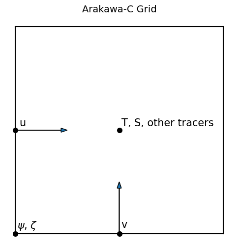
Arakawa and Lamb [1977] define five different grid configurations lettered A-E. Here, the “Arakawa-C” is defined because it is used in MITgcm.

Arakawa-C Grid

The C-grid defines the tracer components at the center of the grid cell and the \(u\)- and \(v\)- velocity components on the left and lower edges of the cell, respectively. With this definition, the stream function (\(\psi\)) and vorticity (\(\zeta\)) are defined on the lower left corner of each cell. We can visualize the grid as follows:

import matplotlib.pyplot as plt

fig = plt.figure(figsize=(6,6))
plt.plot([1,1],[1,2],'k-')
plt.plot([2,2],[1,2],'k-')
plt.plot([1,2],[1,1],'k-')
plt.plot([1,2],[2,2],'k-')

# tracer location
plt.plot([1.5],[1.5],'k.',markersize=14)
plt.text(1.51,1.51,'T, S, other tracers', va='bottom', ha='left', fontsize=15)

# u location
plt.plot([1],[1.5],'k.',markersize=14)
plt.text(1.02,1.51,'u', va='bottom', ha='left', fontsize=15)
plt.arrow(1,1.5,0.25,0, length_includes_head = True, head_width=0.02)

# v location
plt.plot([1.5],[1],'k.',markersize=14)
plt.text(1.51,1.02,'v', va='bottom', ha='left', fontsize=15)
plt.arrow(1.5,1,0,0.25, length_includes_head = True, head_width=0.02)

# stream function and vorticity
plt.plot([1],[1],'k.',markersize=14)
plt.text(1.01,1.01,'$\psi$, $\zeta$', va='bottom', ha='left', fontsize=15)
plt.arrow(1.5,1,0,0.25, length_includes_head = True, head_width=0.02)

plt.title('Arakawa-C Grid',fontsize=14)
plt.axis('off')
plt.show()