The most intuitive type of data collected by satellites is optical imagery - measurements of electromagnetic radiation reflected or emitted from the Earth in visible or near-visible (infrared) portions of the electromagnetic spectrum. Optical imagery is typically collected by passive sensors meaning they rely on energy provided by the sun, rather than emitting their own energy to illuminate the Earth’s surface. On this page, we will explore the data collected by satellites and see a few examples of publicly available satellite products.
To begin, let’s import some Python packages to enable our exploration:
from PIL import Image
import numpy as np
import matplotlib.pyplot as plt
Images and Data
Before diving into some optical satellite data, first let’s explore the organization of a typical image storing data. This will provide some context for the organization of optical satellite data.
Digital Images
Images stored in a digital format are stored with 3-4 numbers describing the constituent colors that make up a given color we see. For example, consider the following image of the progress pride flag, which we read in with PIL and numpy:
# read in the image
im = Image.open('../images/progress_pride_flag.jpg')
im = np.asarray(im)

# show the image with its size
fig = plt.figure(figsize=(4,3))
C = plt.imshow(im)
plt.axis('off')
plt.title('Image Shape: '+str(np.shape(im)))
plt.show()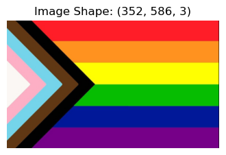
As we can see in the plot above, the progress_pride_flag.jpg image is stored with three dimensions: the number of pixels in the x- and y-directions (586 and 352, respectively) as well as a third dimension for each constitutent color. For jpg images, these layers correspond to the red, green, and blue colors used to make up the colors on a computer screen. Other coloring schemes use different types of color combinations - for example, printers use cyan, magenta, and yellow (and black) to construct colors in a similar fashion. We can observe these constituent colors by plotting their intensity represented as an 8 bit number (0-255) individually as follows:
plt.figure(figsize=(10,3))

plt.subplot(1,3,1)
C = plt.imshow(im[:,:,0],cmap='Greys_r',vmin=0, vmax=255)
plt.axis('off')
plt.colorbar(C,pad=0.04,orientation='horizontal')
plt.title('Red')

plt.subplot(1,3,2)
C = plt.imshow(im[:,:,1],cmap='Greys_r',vmin=0, vmax=255)
plt.axis('off')
plt.colorbar(C,pad=0.04,orientation='horizontal')
plt.title('Green')

plt.subplot(1,3,3)
C = plt.imshow(im[:,:,2],cmap='Greys_r',vmin=0, vmax=255)
plt.axis('off')
plt.colorbar(C,pad=0.04,orientation='horizontal')
plt.title('Blue')

plt.show()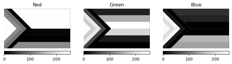
Optical Satellite Images
Much like digital images, satellite images are composed of separate layers called bands that store information about a given scene. However, unlike digital images using red, green, and blue pixel values to reconstruct a given image, optical satellite images are composed of measured reflectances and/or radiances at different wavelengths of the electromagnetic spectrum.
As an example, let’s look at 10 bands measured on 1 June 2024 by the Landsat 8 satellite over the Monterey Bay area in California:
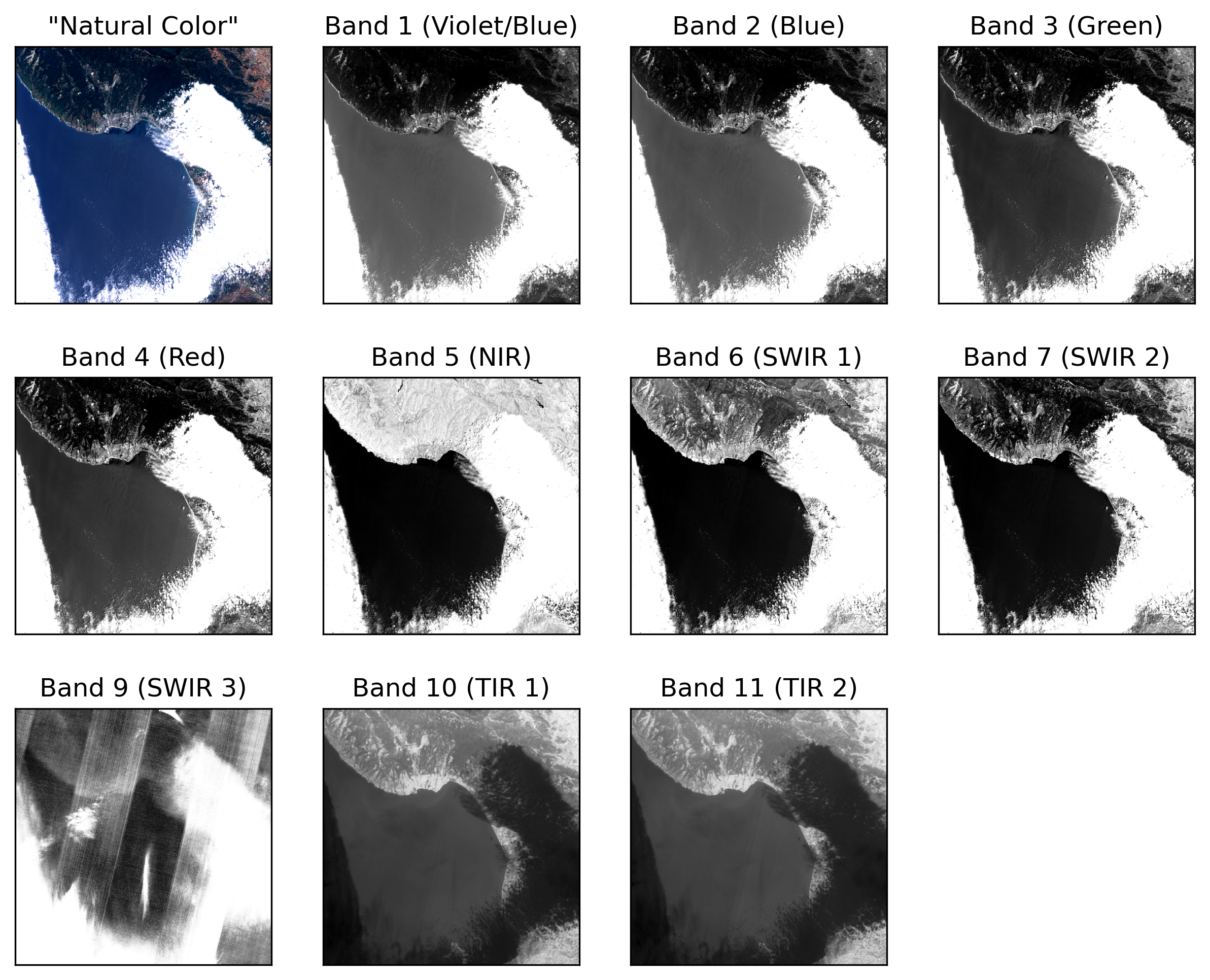
In the above set of images, we can see a “Natural Color” image of the scene showing Monterey Bay in the center in blue, the Santa Cruz mountains to the north in dark green, and an all-too-common scenario for residents of Monterey Bay: a band of coastal fog enshrouding Monterey to the south as well as Salinas and Watsonville to the east.
By looking at the individual bands (summarized below), we can see differences in reflectances and radiances between the different wavelengths. Unsurprisingly, bands 2-4 look similar to the “Natural Color” image since they were used to construct it. However, we start to see differences moving into the near- and shortwave-infrared where the land appears much lighter than the ocean due to the relatively higher reflection of shortwave infrared from land compared to the ocean, which absorbs light in this part of the spectrum. In the shortwave bands, the low-level clouds remain brighter than the ocean and land. Band 9, also in the shortwave infrared, shows evidence of a processing artifact. Bands 10 and 11, both thermal infrared bands as discussed in the next section, show differences in the low clouds - at these wavelengths, low level clouds emit thermal radiation with color clouds emitting less than warmer clouds or other surfaces. As a result, the land and ocean, both of which emit infrared energy, appear brighter than the areas covered by low-level clouds. Note that band 8 is not depicted as it is a panchromatic band.
This collection of images showcases the richness of information and physical processes that can be inferred from optical imagery.
Optical Imagery Satellites
Optical imagery is one of the most common types of data collected by satellites. As a result, there are many different types of optical data with varying resolution and purposes. Here, we detail three U.S. satellite programs with optical sensors.
Landsat
The Landsat mission launched its first satellite in 1972 and has continued until present day. More information about these satellites can be found on the following page.
Aqua and Terra
In 1999, NASA launched its Terra satellite which carries the Moderate Resolution Imaging Spectrometer (MODIS) instrument. The launch of Terra was followed by Aqua in 2002, an similar satellite that also carries MODIS. Both satellites orbited for more than 20 years in a sun-synchronous orbit, imaging a wide range of the Earth’s surface each day. Terra and Aqua remain active missions but are planned for decommissioning in 2026 or 2027.
MODIS has a spatial resolution of 250 m in the red band and 500 m in the blue and green bands, which is roughly 10 times more coarse than Landsat. However, MODIS has a much quicker repeat-pass orbit such that it provides near-global coverage every 1-2 days. More information about the data from these two satellites is discussed in the Ocean Color section, as they have been used to generate global estimates of chlorophyll-a and other biogeochemical variables.
GOES-West
NOAA operates a fleet of Geostationary Operational Environmental Satellites (GOES) that continuously monitor locations in the western hemisphere. The GOES-West satellite is centered over the Pacific Ocean and can be used for monitoring of conditions on the west coast of the United States. The GOES-West imagery has a spatial resolution of 500 m in the red band and 1 km in the blue band (but lacks a green band). Real-time data is available on the National Environmental Satellite, Data, and Information Service site HERE.