Learning Objectives: By the end of this lab, you should be able to
Identify and obtain Landsat imagery in a time and region of interest
Add raster layers to a map and modify their appearance
Identify source projections for vectors and reproject them to new coordinate systems
Mask raster layers with shapefiles
Motivation
When making maps, we often want to use two or more raster files from separate sources. In oceanography, a common scenario is that we have some information in a raster over the ocean and other information in a different raster file over the land - for example, perhaps we want to show the bathymetry of a given region relative to different towns or land features. See, for example, the following screenshot from Google Earth:
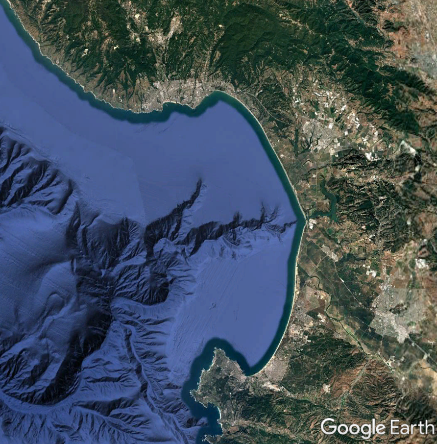
Figure 1:Screenshot of the bathymetry and natural color imagery of the Monterey Bay area shown on Google Earth.
Part 1: Accessing Individual Landsat Scenes
For the land imagery in this lab, we’ll explore how to download Landsat scenes from EarthExplorer and create “Natural Color” images in QGIS. The EarthExplorer portal, hosted by the U.S. Geological Survey (USGS), is a convenient tool to search for available Landsat imagery (as well as data from a variety of other satellites). Navigate to the portal using the link above and sign in with your EROS credentials.
Identifying Landsat Images for your Region of Interest
The EarthExplorer portal is formatted with four panels to narrow down your data search. We’ll walk through each panel here:
Step 1: Search Criteria
The first tab for the search criteria is designed to identify the location and time for your query. For this lab, start by choosing a location in the Monterey Bay area (the “Region of Interest” or “ROI”). The easiest way to identify a location for your data search is to simply click on the map to add a location. If the location is not ideal, delete it and add a new one. If desired, you can also choose a timespan of interest (the default is all available data for your source). Once you’re happy with the query, click Data Sets to continue.
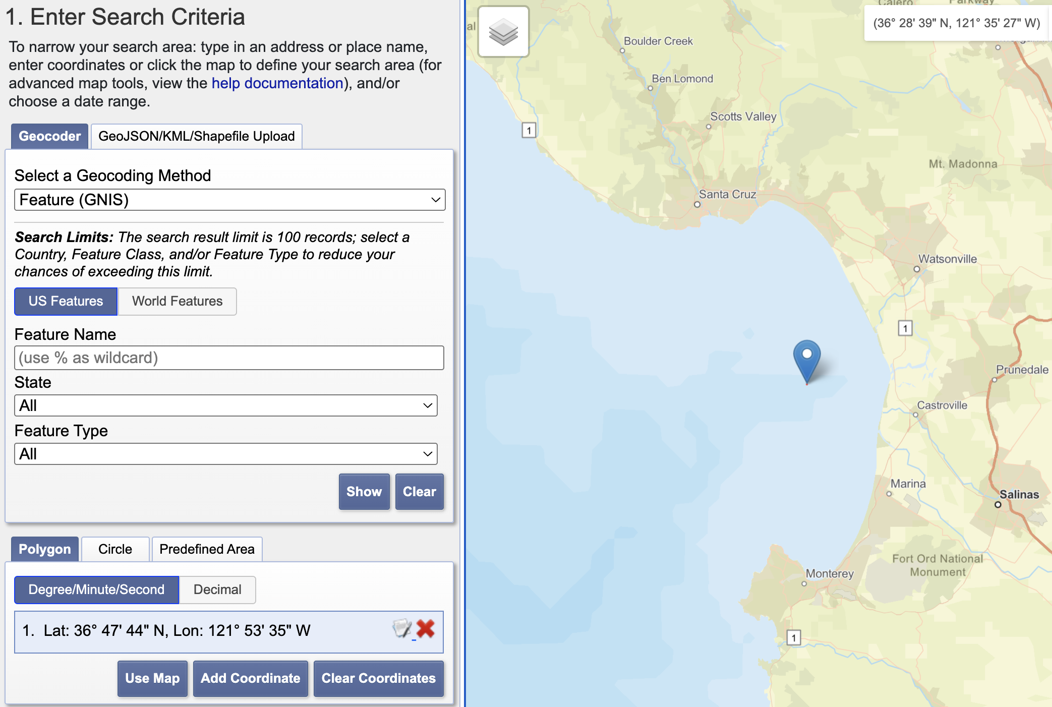
Figure 2:Screenshot of the Monterey Bay query in EarthExplorer.
Step 2: Data Sets
On the Data Sets tab, you’ll find that there are lots of different options available for different types of data. Scroll down through the list of sensors and expand the Landsat menu and choose Landsat Collection 2 Level 2 for imagery. For recent imagery, choose the set pertaining to Landsat 8-9 OLI/TIRS CS L2. Then click Results to view the options (you can skip the Additional Criteria tab).
Step 3: Downloading Data
On the Results page, you’ll get a list of available Landsat images that span the Monterey Bay area. Scroll through the available options and consider the following question:
Is the image from Landsat 8 or Landsat 9?
What is the approximate temporal spacing between the images?
Are there clouds in the image? (Hint: you can get a closer look at the image by clicking on the thumbnail of the image)
After browsing the images, choose a relatively cloud-free image of your ROI. Once you have identified an image, download the Blue, Green, and Red Bands for your scene by clicking on the Download button (grey disk with the green arrow). Since we’re working with Landsat 8 and 9, these bands are B2, B3, and B4. For Landsat 4-5, these would be bands B1, B2, and B3.
To download the individual bands, click on the bands in the expanded menu for the Level-2 Surface Reflectance Bands:
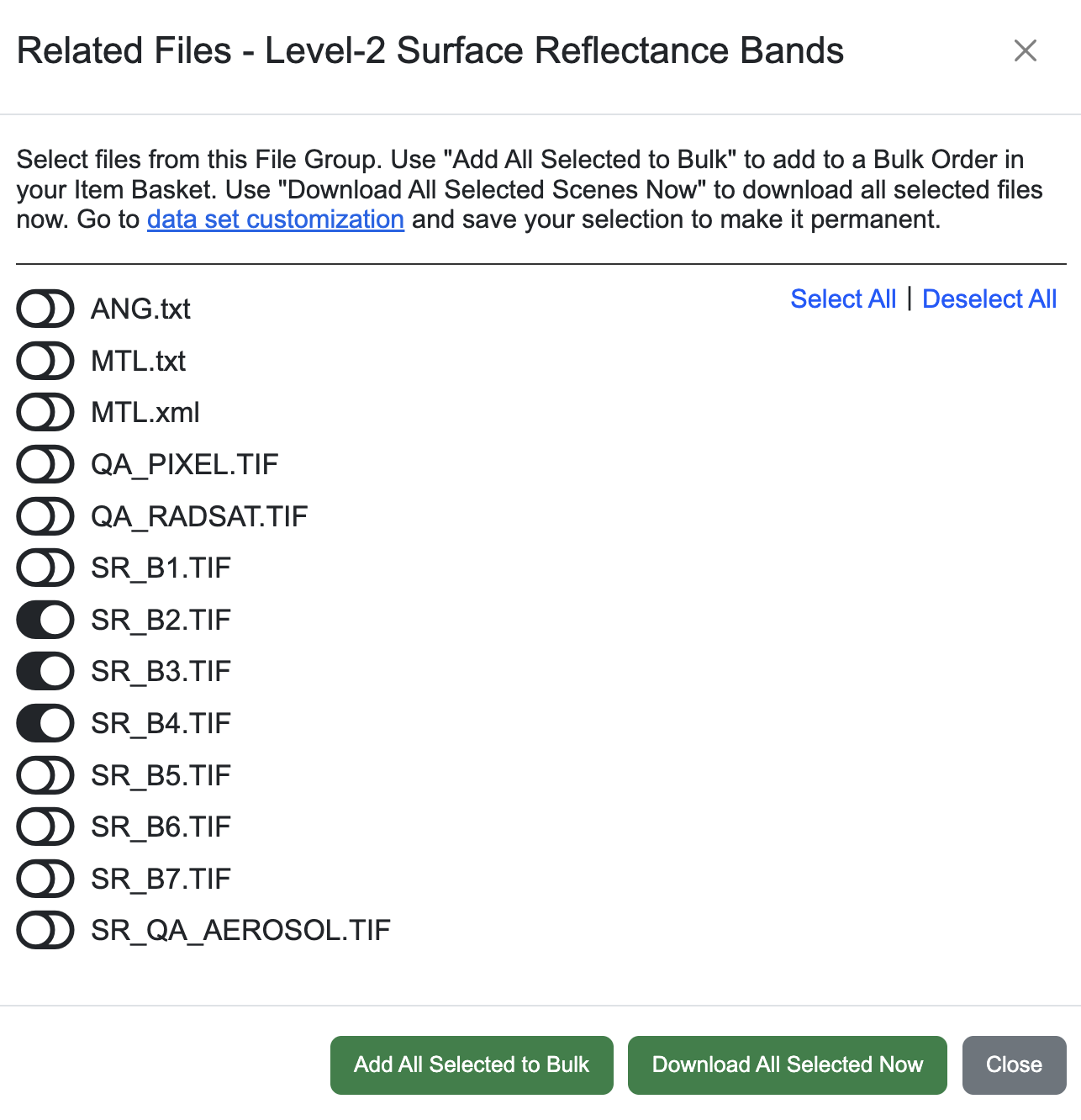
Figure 1:Screenshot of the bathymetry and natural color imagery of the Monterey Bay area shown on Google Earth.
Part 2: Creating a “Natural Color” Landsat Image in QGIS
To generate a “Natural Color” image in QGIS, it’s necessary to “merge” the Red, Green, and Blue Landsat bands into a single image and then render the image accordingly.
Merge the Image in QGIS
From the Raster drop-down, choose Miscellaneous → Merge
Click the option to Place each input file into a separate band
In the Input Layers tab, choose to Add Files... and add the files for the blue (B2), green (B3), and red (B4) bands
Save the file as a GeoTIFF (
tif) file with the suffix “Natural”
Assign Bands to the Correct Colors
When your merged image is loaded into QGIS, open up the Properties menu and change the bands so that the red band is assigned to band 3, green to band 2, and blue to band 1 (if they are not ordered in this way)
It is often helpful to scale the colors to the same numerical extent
Render the Image
Under the Properties tab for your layer, adjust the contrast, brightness, saturation, and gamma levels to visualize the image as desired. Here are some suggestions:
In the Transparency tab, add a 0 value to the transparency (this will remove the black points on the edges)
Change the “stretching” of the Red, Green, and Blue bands either manually (perhaps in the range 5000-14000) or by calculating a stretch using the Stretch to MinMax option with min and max values set by the Cumulative Count Cut
Increase the Gamma values and Brightness values from their default values.
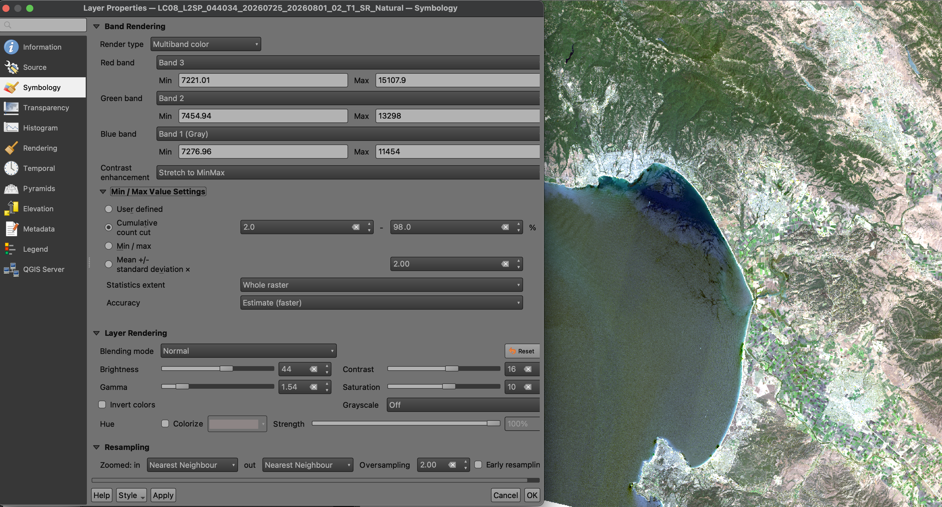
Figure 4:Screenshot of the Surface Reflectance Bands download menu.
Part 3: Clipping a Vector Layer to the Map Extent
In subsequent steps, we are going to use our coastline vector layer to mask out the ocean component of the Landsat. Begin by adding the global coastline shapefile we obtained in the previous lab (the GSHHS layer).
We will use a clipping tool to mask out the Landsat data over the ocean. However, this tool will make a new raster layer as large as the vector layer – in our case, if we use the global coastline layer from the previous lab, this is the whole globe! That file would be huge. To circumvent that issue, we will first make a smaller version of our coastline layer by clipping the layer to the map extent.
Start by ensuring your projection is in the same coordinates as the coastline layer (EPSG: 4326) by looking in the bottom-right corner of the QGIS screen. If it indicates another projection (e.g. EPSG: 32610) then click on this projection and change it to EPSG 4326.
Next, open up the “Clip vectors by extent” tool. You can find this tool as follows: - Open the Processing Toolbox by clicking on View → Panels → Processing Toolbox - Under GDAL → Vector geoprocessing, find the Clip vectors by extent tool
To clip the layer, choose the Input layer to be the Global Coastline shapefile. Then, under Clipping extent, choose Use Current Map Canvas Extent. You can save as a permanent layer if you’d like, or you can save as a temporary layer since we will make one more modification in the next step.
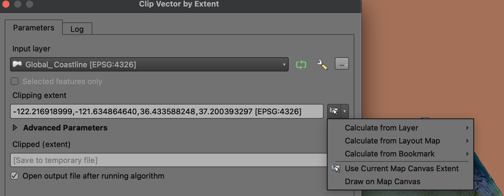
Figure 5:Screenshot of the Clip Layer by Extent tool.
Part 4: Reprojecting Vector Layers
When using layers for calculations in GIS, it is crucial that the underlying data are in the same coordinate system. Right now, our coastline layer is in one projection (4326) while our satellite data is in another (UTM coordinates). This is fine for visualization, but not for calculations.
You can check the coordinate system of a layer by right-clicking on the layer and opening the Properties menu. Under the Source tab, there is a section for the Coordinate Reference System (CRS). Note that this CRS can be (and often is) different than the CRS of the map – in fact, one map can have layers spanning a variety of different coordinate systems.
To reproject a layer, we need to create an entirely new file – the database file stores the data into a set of points that are specific to the CRS in use. It is not enough to just change the assigned CRS in the properties tab.
Here, we will reproject the vector layer into the projection of the Landsat layer. Begin by identifying the projection of your Landsat Layer. Right-click on the “Natural” layer and choose Properties... Then, click on the Source tab and note the CRS.
Next, reproject your vector by right-clicking on the clipped coastline layer and choose Export → Save Features As. For the File name, save this layer as the same name as your previous layer but add the CRS code to the end (e.g. Monterey Coastline 36210.shp). Then, Change the CRS of the layer to the same one as your Landsat Layer and click OK. This will generate a new layer on your map that looks identical to the previous one - but the underlying data will now be saved in the new coordinates.
Part 5: Clipping Raster Layers
In the previous part, we created a coastline layer in the same projection as our Landsat raster layer. Next, we will “clip” our raster layer to mask out the ocean, allowing us to see the bathymetry layer underneath.
Open the Clip Raster By Mask Layer tool, available under Raster → Extraction drop-down menu
For the Input layer, choose your Natural Color Landsat layer
For the Mask layer, use your reprojected clipped vector layer
Choose a file name and location where you will store your new layer
Hit Run!
On your Canvas, you should now have a smaller version of your Landsat file which has the ocean area removed. Reformat your new Landsat layer using the Properties menu as before. If you’d like the same style as the previous layer, you can right-click on the original Landsat layer and choose Style → Copy Style. Then, on the new layer, choose Style → Paste Style.
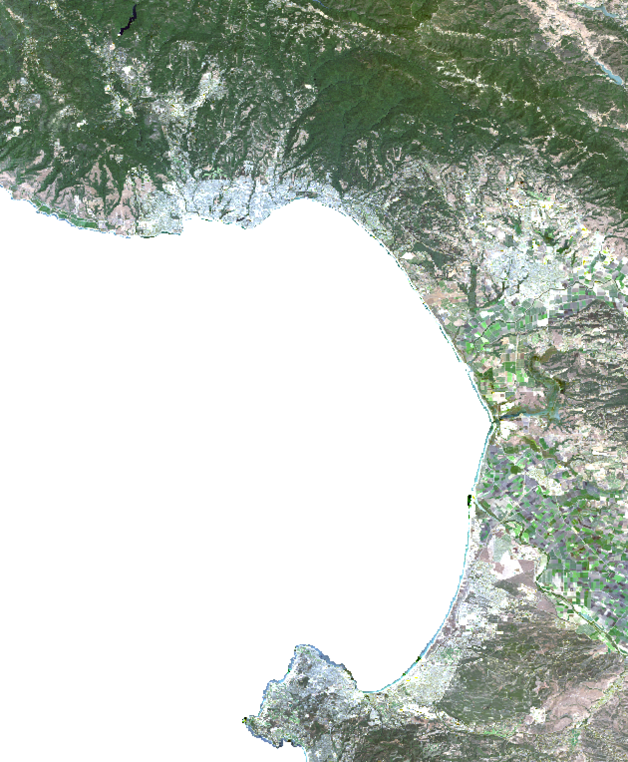
Figure 6:Screenshot of a “Natural Color” Landsat scene with the ocean clipped out.
🤔 Try it for yourself!
Try the following two steps to practice your QGIS skills:
Revisit the map you made in Lab 1. Add your new Landsat imagery layer and create a new figure with both bathymetry and a “natural” scene on land, similar to the rendering on Google Earth.
Create another map to investigate changes in your region – say between seasons or over many years. Follow the instructions above to recreate another clipped Landsat image of the region for a different time. Make a figure showing the two scenes side-by-side to visualize the differences. Be sure to copy the style of the first scene to the second so that both scenes look the same.