Single-Layer Perceptrons from Scratch - Introduction to Machine Learning

In this notebook, we revisit our perceptron classification model for a multi-class problem. This will give us a framework to explore more complex models down the road in a model structure called a neural network.

Learning Objectives

Implement a perceptron for multi-class classifications of multidimensional data.
Compute the gradient of a multi-dimensional loss function for use in a perceptron.
Implement a single-layer perceptron in a Python class.

Import modules

Begin by importing the modules to be used in this notebook.

import os
import numpy as np
import matplotlib.pyplot as plt
import pandas as pd
import struct

The MNIST Dataset¶

In this notebook, we will examine a dataset of handwritten digits from the Modified National Institute of Standards and Technology (MNIST) dataset. The MNIST Dataset is like the “Hello World” of neural network data.

Let’s create a quick function to read in the images and the labels in either the testing or the training data:

def read_mnist_images(data_directory, subset='train'):
    if subset=='train':
        prefix = 'train-'
    else:
        prefix = 't10k-'
        
    with open(os.path.join(data_directory,'MNIST',prefix+'images.idx3-ubyte'), 'rb') as f:
        # unpack header
        _, num_images, num_rows, num_cols = struct.unpack('>IIII', f.read(16))
        
        # read image data
        image_data = f.read(num_images * num_rows * num_cols)
        images = np.frombuffer(image_data, dtype=np.uint8)
        images = images.reshape(num_images, num_rows, num_cols)

    with open(os.path.join(data_directory,'MNIST',prefix+'labels.idx1-ubyte'), 'rb') as f:
        # unpack header
        _, num_labels = struct.unpack('>II', f.read(8))

        # read label data
        labels = np.frombuffer(f.read(), dtype=np.uint8)

        
    return images, labels

We can use this function as follows:

# load in the training and test images
train_images, train_labels = read_mnist_images('../data','train')
test_images, test_labels = read_mnist_images('../data','test')

# print the sizes
print('Training Image Set Size: ',np.shape(train_images))
print('Testing Image Set Size: ',np.shape(test_images))
print('Training Label Set Size: ',np.shape(train_labels))
print('Testing Label Set Size: ',np.shape(test_labels))

Training Image Set Size:  (60000, 28, 28)
Testing Image Set Size:  (10000, 28, 28)
Training Label Set Size:  (60000,)
Testing Label Set Size:  (10000,)

We can see that this set contains 60,000 training images sized 28x28 and a testing set with 10,000 images of the same size. Let’s take a look at what these images looks like:

# choose a set of indices 
np.random.seed(14)
test_indices = np.random.randint(low=0, high=10000, size=10)

# make a plot of the predictions
plt.figure(figsize=(10,6))
for d, index in enumerate(test_indices):
    plt.subplot(2,5,d+1)
    plt.imshow(train_images[index,:,:],cmap='Greys')
    plt.title('True Label: '+str(train_labels[index]))
    # plt.axis('off')
plt.show()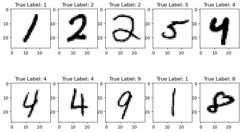

As we can see, each image is a 28 pixel x 28 pixel image of a hand-written digit.

The Single-Layer Perceptron¶

In our previous lessons on classification, we came across the Perceptron. Here, we will revisit this approach to build a model to classify the hand-written images.

One-Hot Encoding¶

In our previous example of a Perceptron, we used a single vector to represent our target classifications (0 for no, 1 for yes). Here, we are going to employ a slightly different encoding called a one-hot encoding. This will be a set of column vectors - one for each class - that identifies whether the image corresponds to that class.

Let’s see how that works - for example, for the number 4:

# compute the one-hot encoding
one_hot = np.zeros((train_labels.shape[0], 10)).astype(int)
for i, val in enumerate(train_labels):
    one_hot[i, val] = 1
    
print('First 5 labels:')
print(train_labels[:5])
print('\nFirst 5 encodings:')
print(one_hot[:5,:])

First 5 labels:
[5 0 4 1 9]

First 5 encodings:
[[0 0 0 0 0 1 0 0 0 0]
 [1 0 0 0 0 0 0 0 0 0]
 [0 0 0 0 1 0 0 0 0 0]
 [0 1 0 0 0 0 0 0 0 0]
 [0 0 0 0 0 0 0 0 0 1]]

As we can see, the one-hot encoding has a value of 1 corresponding to the index of the label (0–9). For example, when the label is 5, all values are 0 except for the value at index 5.

The Forward Model¶

In this model formulation, we will create our model to read in an “unraveled” image (or a set of them). That is, instead of reading in images sized 28x28, we will reshape them so that the image sizes are one vector of length 784 (= 28*28).

X_train = train_images.reshape(-1, 784) / 255.0
X_test = test_images.reshape(-1, 784) / 255.0
Y_train = train_labels
Y_test = test_labels

print('Training Image Set Size: ',np.shape(X_train))
print('Testing Image Set Size: ',np.shape(X_test))
print('Training Label Set Size: ',np.shape(Y_train))
print('Testing Label Set Size: ',np.shape(Y_test))

Training Image Set Size:  (60000, 784)
Testing Image Set Size:  (10000, 784)
Training Label Set Size:  (60000,)
Testing Label Set Size:  (10000,)

Each pixel - 784 in total - will be assigned its own individual weight in the network which will be combined in a linear combination along with a bias unit yielding a total of 10 model labels. After these values are determined, the linear combination will be passed to a sigmoid activation function as we saw in our lesson on Logistic Regression to rescale the model output. The following diagram depicts the forward model. In this example, we trace through the network to follow the calculation for the probability that the image is a 2:

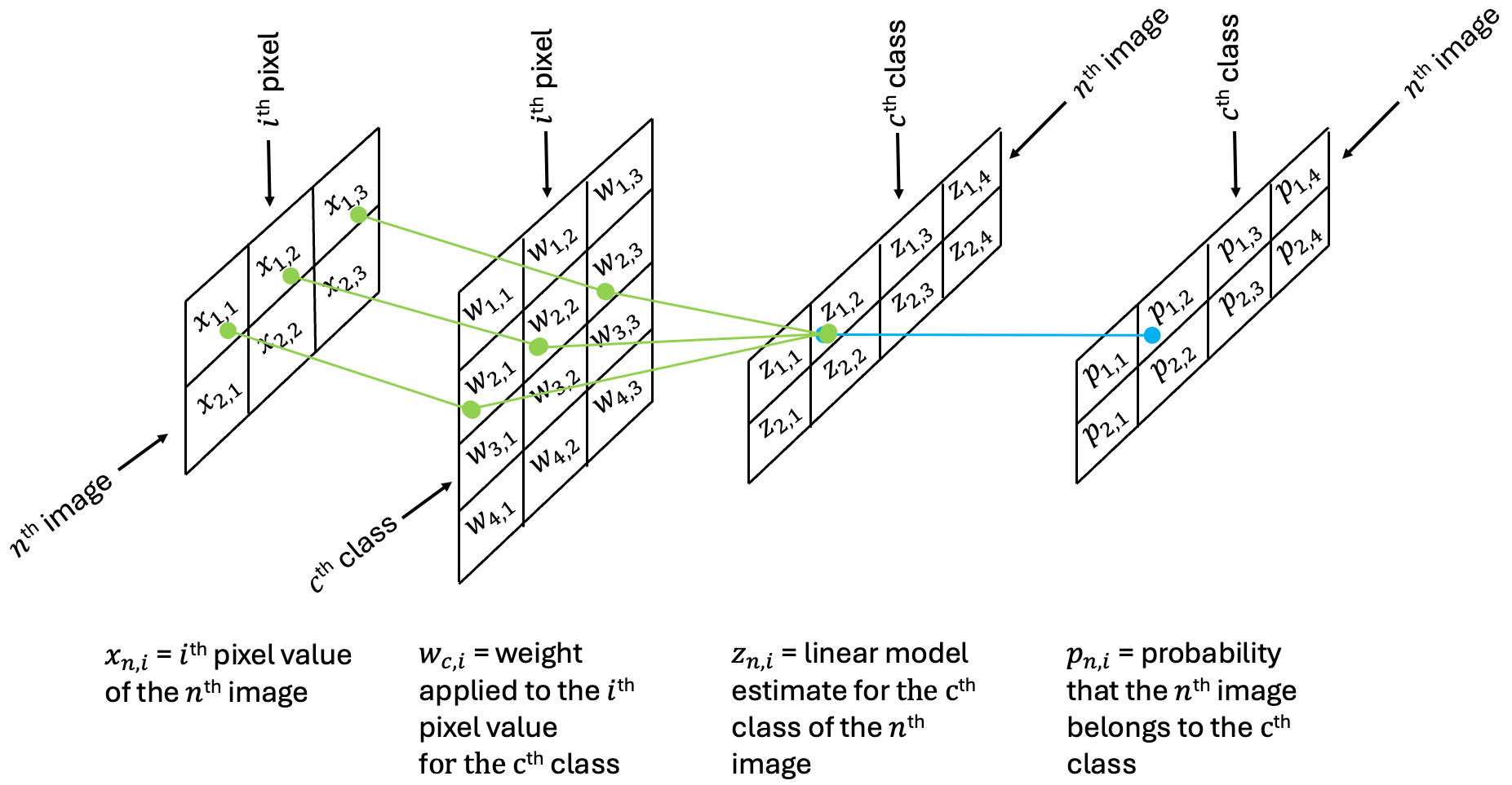
\begin{align*} z &= Xw^T+b \\ p &= \sigma(z) \end{align*}

(1)

In the implementation here, it is important to note the sizes of each matrix in terms of the rows and columns:

X: (N, I)
w: (C, I)
z: (N, C)
p: (N, C)

In the schematic above, N=2, C=4, and I=2. In the MNIST image example, N=60000, C=10, and I=784.

A Note on Neurons¶

The diagram above is an example of an artificial neuron for its relation to how neurons in our human brains operate. Neurons in the brain receive electrical signals (err.. computations) from the nervous system. Based on the character of these signals, a neuron will either “fire” or not - that is, it will either pass on information or it won’t. The simple perceptron model replicates this procedure. A set of input data (one row of the image) is passed to the neuron (via a linear combination of weights and the bias) and the activation function determines how the information is passed (in the form of a probability). The output of this neuron is then provided to make a simple decision (not shown above). In this case, the classification will depend on the highest probability value. However, in other applications, the output of the neuron may be passed to other neurons. In this sense, we can build a “neural network” which is composed of a series of perceptron-like models that allow highly non-linear decision making. We’ll see examples of this in the notebooks to come. For now, let’s take a look at optimizing the weights of our perceptron here.

The Loss Function¶

To compute the optimal weights for our model, we’ll need to define a loss function. Here, we will use the mean square error loss function:

L = \frac{1}{NC} \sum_{n=1}^N \sum_{c=1}^C (y_{n,c}-p_{n,c})^2

(2)

Here, the loss is computed across all of the $N$ images (60,000 in this case) and all of the $C$ classes (10 in this case). Note that there are more ideal loss functions for this task but the mean square error loss function will keep the derivations below more familiar.

The Derivative of the Loss Function¶

To use the gradient descent algorithm, we first need to compute the derivatives of the loss function with respect to the weights. Each of our image pixels has a collection of 10 individual weights - one for each of the classifications. This means we will have a 2D matrix of weights, sized (10, 784) in this case.

As we see above, $L$ is a function of $p_{n,c}$ (the probability that the nth image belongs to class $c$ ) which in turn is a function of $z_{n,c}$ (the linear model estimate of the nth image for class $c$ ), which is in turn a function of the weights and the biases. The chain rule provides a way to compute these weights. This process of tracing back the derivatives through the model network is called back propagation.

A small example¶

Before deriving the full gradient of the loss function, I find it easiest to consider a smaller example with the shapes shown in the schematic above. Writing out the loss explicitly, we have

\begin{align*} L = \frac{1}{8} [ &(y_{1,1} - p_{1,1})^2 + (y_{1,2} - p_{1,2})^2 + (y_{1,3} - p_{1,3})^2 + (y_{1,4} - p_{1,4})^2 \\ &(y_{2,1} - p_{2,1})^2 + (y_{2,2} - p_{2,2})^2 + (y_{2,3} - p_{2,3})^2 + (y_{2,4} - p_{2,4})^2] \end{align*}

(3)

Now, considering computing the gradient with respect to a given weight - say $w_{2,3}$ - which is applied to the third index to compute the probability the image belongs to the second class. Looking at the diagram above, we see that that the only $p_{1,2}$ and $p_{2,2}$ depend on this weight, so the gradient becomes

\begin{align*} \dfrac{\partial L}{\partial w_{2,3}} &= \frac{-2}{8} \left[ (y_{1,2} - p_{1,2}) \frac{\partial p_{1,2}}{\partial z_{1,2}} \frac{\partial z_{1,2}}{\partial w_{2,3}} + (y_{2,2} - p_{2,2}) \frac{\partial p_{2,2}}{\partial z_{2,2}} \frac{\partial z_{2,2}}{\partial w_{2,3}} \right] \\ &= \frac{-2}{8} \left[ (y_{1,2} - p_{1,2}) p_{1,2}(1-p_{1,2})x_{1,3} + (y_{2,2} - p_{2,2}) p_{2,2}(1-p_{2,2})x_{2,3} \right] \end{align*}

(4)

Note that we are using the following formula derived in the Logistic Regression notebook:

\dfrac{\partial p_{n,c}}{\partial z_{n,c}} = p_{n,c}(1-p_{n,c})

(5)

If we define

\mathcal{D}_{n,c} = -2(y_{n,c} - p_{n,c}) p_{n,c}(1-p_{n,c})

(6)

Then we can write this as

\dfrac{\partial L}{\partial w_{2,3}} = \frac{1}{8} \sum_{n=1}^2 \mathcal{D}_{n,2} x_{n,3}

(7)

Generalizing to each of the individual weights, we have

\dfrac{\partial L}{\partial \textbf{w}} = \frac{1}{8}\begin{bmatrix} \sum_{n=1}^2 \mathcal{D}_{n,1} x_{n,1} & \sum_{n=1}^2 \mathcal{D}_{n,1} x_{n,2} & \sum_{n=1}^2 \mathcal{D}_{n,1} x_{n,3} \\ \sum_{n=1}^2 \mathcal{D}_{n,2} x_{n,1} & \sum_{n=1}^2 \mathcal{D}_{n,2} x_{n,2} & \sum_{n=1}^2 \mathcal{D}_{n,2} x_{n,3} \\ \sum_{n=1}^2 \mathcal{D}_{n,3} x_{n,1} & \sum_{n=1}^2 \mathcal{D}_{n,3} x_{n,2} & \sum_{n=1}^2 \mathcal{D}_{n,3} x_{n,3} \\ \sum_{n=1}^2 \mathcal{D}_{n,4} x_{n,1} & \sum_{n=1}^2 \mathcal{D}_{n,4} x_{n,2} & \sum_{n=1}^2 \mathcal{D}_{n,4} x_{n,3} \end{bmatrix}

(8)

In one more rearrangement, we can write the above matrix as a multiplication of the following:

\dfrac{\partial L}{\partial \textbf{w}} = \begin{bmatrix} \mathcal{D}_{1,1} & \mathcal{D}_{2,1} \\ \mathcal{D}_{1,2} & \mathcal{D}_{2,2} \\ \mathcal{D}_{1,3} & \mathcal{D}_{2,3} \\ \mathcal{D}_{1,4} & \mathcal{D}_{2,4} \end{bmatrix} \begin{bmatrix} x_{1,1} & x_{1,2} & x_{1,3} \\ x_{2,1} & x_{2,2} & x_{2,3} \end{bmatrix} = \mathcal{D}^T \textbf{X}

(9)

Generalizing to an arbitrary size¶

Using the above framework, we can generalize to an arbitrary number of images $N$ , classes $C$ and image length $I$ .

Consider a weight $w_{c,i}$ corresponding to class $c$ and pixel $i$ . We can express the derivative of the loss function for an individual weight as:

\dfrac{\partial L}{\partial w_{c,i}} = \frac{-1}{N} \sum_{n=1}^N 2(y_{n,c}-p_{n,c}) p_{n,c}(1-p_{n,c}) x_{n,i}

(10)

Here, for simplicity, I will drop the constant term since it can be absorbed into the learning rate.

Written out in complete matrix form we can express the full gradient following the structure above:

\begin{align*} \dfrac{\partial L}{\partial \textbf{w}} &= \frac{-2}{N} \begin{bmatrix} (y_{1,1}-p_{1,1}) p_{1,1}(1-p_{1,1}) & \cdots & (y_{N,1}-p_{N,1}) p_{N,1}(1-p_{N,1}) \\ & \ddots & \\ (y_{1,C}-p_{1,C}) p_{1,C}(1-p_{1,C}) & \cdots & (y_{N,C}-p_{N,C}) p_{N,C}(1-p_{N,C})\end{bmatrix} \begin{bmatrix} x_{1,1} & \cdots & x_{1,I} \\ & \ddots & \\ x_{N,1} & \cdots & x_{N,I}\end{bmatrix} \\ &= \mathcal{D}^T \textbf{X} \end{align*}

(11)

where, again for clarity, here we have defined the following matrix:

\mathcal{D} = \frac{2}{N} \begin{bmatrix} (y_{1,1}-p_{1,1}) p_{1,1}(1-p_{1,1}) & \cdots & (y_{1,C}-p_{1,C}) p_{1,C}(1-p_{1,C}) \\ & \ddots & \\ (y_{N,1}-p_{N,1}) p_{N,1}(1-p_{N,1}) & \cdots & (y_{N,C}-p_{N,C}) p_{N,C}(1-p_{N,C})\end{bmatrix}

(12)

Coding Up a Solution¶

Now that we know how to compute our gradients, let’s write some code to create our model!

class SingleLayerPerceptron:

    def __init__(self, num_features, num_classes, random_seed=123):
        self.num_classes = num_classes
        generator = np.random.RandomState(random_seed)
        self.weight_out = generator.normal(loc=0.0, scale=0.1, size=(num_classes, num_features))
        self.bias_out = np.zeros(num_classes)

    def int_to_onehot(self, y, num_labels):
        ary = np.zeros((y.shape[0], num_labels))
        for i, val in enumerate(y):
            ary[i, val] = 1
        return(ary)

    def sigmoid(self,z):
        return 1 / (1 + np.exp(-np.clip(z, -250, 250))) # clipping prevent overflows

    def forward(self, x):
        z_out = np.dot(x, self.weight_out.T) + self.bias_out
        a_out = self.sigmoid(z_out)
        return(a_out)

    def predict(self, X):
        probs = self.forward(X)
        return np.argmax(probs, axis=1)

    def backward(self, x, a_out, y):
        y_onehot = self.int_to_onehot(y, self.num_classes)

        # compute the components of the derivative of the loss function
        # first the weights
        d_L__d_p = 2*(a_out - y_onehot)/y.shape[0]
        d_a_out__d_z_out = a_out * (1-a_out) 
        D = d_L__d_p * d_a_out__d_z_out
        d_z_out__d_w_out = x
        d_loss__d_w_out = np.dot(D.T, d_z_out__d_w_out)
        # then the bias
        d_loss__d_b_out = np.dot(D.T, np.ones_like(y))

        return(d_loss__d_w_out, d_loss__d_b_out)

    def mse_loss(targets, probs, num_labels=10):
        onehot_targets = self.int_to_onehot(targets, num_labels)
        err = np.mean((onehot_targets - probs)**2)
        return(err)

    def compute_mse_and_acc(self, X, y, num_labels=10):
        probs = self.forward(X)
        predicted_labels = np.argmax(probs,axis=1)
        onehot_targets = self.int_to_onehot(y, num_labels)
        loss = np.mean((onehot_targets - probs)**2)
        acc = np.sum(predicted_labels == y)/len(y)
        return(loss, acc)

    def train(self,X_train, Y_train, X_test, Y_test, num_epochs, learning_rate=0.1):
        train_losses = []
        test_losses = []
        train_accs = []
        test_accs = []
        for e in range(num_epochs):

            #forward method
            a_out = self.forward(X_train)

            # backward method
            d_loss__d_w_out, d_loss__d_b_out = self.backward(X_train, a_out, Y_train)

            # gradient descent
            self.weight_out -= learning_rate*d_loss__d_w_out
            self.bias_out -= learning_rate*d_loss__d_b_out

            # keep track of stats
            train_loss, train_acc = self.compute_mse_and_acc(X_train, Y_train)
            train_losses.append(train_loss)
            train_accs.append(train_acc)
            test_loss, test_acc = self.compute_mse_and_acc(X_test, Y_test)
            test_losses.append(test_loss)
            test_accs.append(test_acc)
        return(train_losses, train_accs, test_losses, test_accs)

Using the Perceptron Model¶

Now that we’ve got the model coded up, let’s train it and use it to classify the images. First, let’s train the model.

slp = SingleLayerPerceptron(784,10)
train_losses, train_accs, test_losses, test_accs = \
 slp.train(X_train, Y_train, X_test, Y_test, 1000, learning_rate=0.5)

As always, we should take a look at the loss functions through the training process:

# plot the losses and accuracies
plt.figure(figsize=(10,5))

plt.subplot(1,2,1)
plt.plot(train_losses,label='Train')
plt.plot(test_losses,label='Test')
plt.ylabel('Loss')
plt.xlabel('Iterations')
plt.legend()

plt.subplot(1,2,2)
plt.plot(train_accs,label='Train')
plt.plot(test_accs,label='Test')
plt.ylabel('Accuracy')
plt.ylim([0,1])
plt.xlabel('Iterations')
plt.show()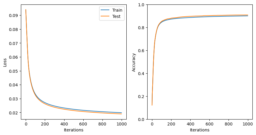

With more than 1000 iterations and a learning rate of 0.5, our model has now started to converge.

Let’s see how it works on a collection of random images:

# choose a set of indices 
np.random.seed(14)
test_indices = np.random.randint(low=0, high=10000, size=10)

# make a plot of the predictions
plt.figure(figsize=(10,6))
for d, index in enumerate(test_indices):
    plt.subplot(2,5,d+1)
    plt.imshow(train_images[index,:,:],cmap='Greys')
    plt.title('True Label: '+str(train_labels[index])+\
              '\n Predicted Label: '+str(slp.predict(train_images[index,:,:].reshape(1, 784))[0]))
    plt.axis('off')
plt.show()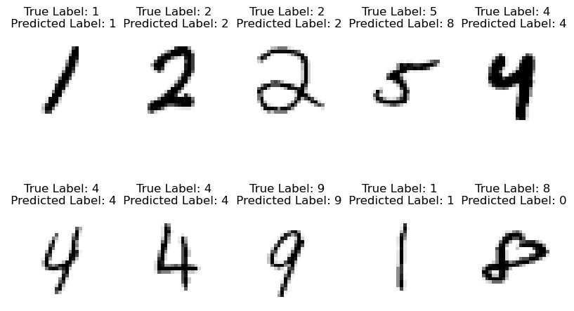

Not bad! But can we do better? Let’s see in the next notebook!

Key Takeaways

In a perceptron, a weight is applied to each individual input feature.
The chain rule provides a mechanism to break down the gradient of the loss function with respect to the weights into individual components.