Logistic Regression - Introduction to Machine Learning

In this notebook, we revisit the classification problem using logistic regression.

Learning Objectives

By the end of this notebook, you should be able to

Explain the formulation of logistic regression and how it is used for classification
Write a Python class to iteratively optimize a logistic regression model
Interpret the results of a logistic regression model after it has been fit to data.

Import modules Begin by importing the modules to be used in this notebook

import os
import numpy as np
import matplotlib.pyplot as plt
import pandas as pd

Classification Revisited¶

In this notebook, we will revisit the classification problems introduced in the Perceptron notebook for sea lions. Let’s read that in again here:

# read in the two data frames
df_female = pd.read_csv(os.path.join('..','data',
                                     'female_sea_lion_measurements.csv')) # Data S1
df_male = pd.read_csv(os.path.join('..','data',
                                    'male_sea_lion_measurements.csv'))     # Data S2

# concatenate the dataframes
df = pd.concat([df_male, df_female])

# drop nans
df = df.dropna()

Similar to our previous exploration, we will add a new column to encode the classification:

# add a classification column
df['Classification'] = 1
df.loc[df['Sex']=='Male', "Classification"] = 0

As a reminder of what the data looks like, let’s make a quick plot:

plt.plot(df['SL'][df['Classification']==0],
         df['CBL'][df['Classification']==0],'b.',label='Class 0 (Male)')
plt.plot(df['SL'][df['Classification']==1],
         df['CBL'][df['Classification']==1],'r.',label='Class 1 (Female)')
plt.xlabel('parameter 1 (body length, cm)')
plt.ylabel('parameter 2 (skull length, mm)')
plt.legend(loc=2)
plt.show()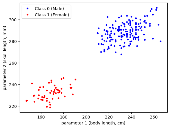

Just as for our previous example, we will work with standardized variables. Let’s create those for our dataset:

df['SL_norm'] = (df['SL'] - np.mean(df['SL']))/np.std(df["SL"])
df['CBL_norm'] = (df['CBL'] - np.mean(df['CBL']))/np.std(df["CBL"])

In addition, let’s define some bounds we will use for plotting:

# define some bounds to be used in the plots below
min_x = -3
max_x = 3
min_y = -3
max_y = 3

Logistic Regression¶

In our previous example with the perceptron, we drew a simple line to distinguish between the two classifications. However, not all solutions to this problem were ideal.

In this example, we are going to model the probability that a given point is associated with a given class. In symbols, we can define the probability $p$ that a given point belongs to class 1 given some input features (x, here, the skull and body length parameters) as

p = p(c=1 | \textbf{x} )

(1)

Given this probability, we can define the odds as $p/(1-p)$ . In logistic regression, it is assumed that the log-odds, also known as the logit function, is related to the input features in a linear way:

\text{logit}(p) = \log\left(\frac{p}{1-p}\right) = b + w_1 x_1 + w_2x_2

(2)

Here, the linear relation is written in terms of two input features but additional features with corresponding weights can be added as well. Since we are interested in the probability $p$ , we need to apply the inverse of the logit function, which is termed the sigmoid function and has the following form:

\sigma (z) = \frac{1}{1+e^{-z}}

(3)

You can try this for yourself to ensure it is indeed the inverse - what happens when you plug the logit function into the sigmoid function?

Writing this explicitly, we generate a model for the probability $p$ by applying the sigmoid function to the equation above yielding:

p = \frac{1}{1+e^{-(b + w_1 x_1 + w_2x_2)}}

(4)

This approach is what’s know as “Logistic Regression”. It is important to note that the name is a little misleading - in linear regression, we fit a linear model to some data. In logistic regression, we are NOT fitting a logistic model to data. Rather, we are modeling membership in a given classes as a probability and assuming an underlying transformation for this relationship.

Deriving gradients for logistic regression¶

In contrast to the previous examples where we would like to minimize a loss function, here we would like to maximize the likelihood function ( $\mathcal{L}$ ) of the weights given the input features. This is given by the product of the probabilities which can be formulated with a Bernoulli distribution as follows:

\mathcal{L}(\textbf{w}|\textbf{x}) = \prod_{i=1}^n p(c^{(i)}|\textbf{x}^{(i)};\textbf{w}) = \prod_{i=1}^n p^{c^{(i)}} (1- p)^{1-c^{(i)}}

(5)

We could construct a gradient descent algorithm using this formula, but a log transform is often applied to the above equation to give the log-likehood function as follows:

\mathcal{l}(\textbf{w}|\textbf{x}) = \sum_{i=1}^n c^{(i)} \log(p) + (1-c^{(i)})\log (1- p)

(6)

As we can see, this allows us to leverage properties of the log function to rewrite the function as a sum and remove some of the exponents - this will make the derivative computations for gradient decent much cleaner. Since the log function is a monotonically increasing function, the maximum of the log-likehood will be equivalent to the maximum of the likehood.

Keeping in line with the previous examples we’ve seen where we minimize a loss function, we can also multiply this function by -1 so that we can employ our typical gradient descent approach to the following loss function:

L = \sum_{i=1}^n -c^{(i)} \log(p) - (1-c^{(i)})\log (1- p)

(7)

Now that we’ve got our function to minimize, we just need to compute our derivatives. Let’s consider our bias term first. When computing the derivative of $L$ , we see that $L$ is a function of $p$ which, in turn, is a function of $b$ , so we must apply the chain rule:

\frac{\partial L}{\partial b} = \frac{\partial L}{\partial p} \frac{\partial p}{\partial b}

(8)

Let’s compute these separately. The first derivative is:

\frac{\partial L}{\partial p} = \sum_{i=1}^n \left(\frac{-c^{(i)}}{p} + \frac{1-c^{(i)}}{1-p}\right) = \sum_{i=1}^n \frac{p-c^{(i)}}{p(1-p)}

(9)

and the second derivative is:

\begin{align*} \frac{\partial p}{\partial b} &= \frac{\partial }{\partial b}\left( (1+e^{-(b + w_1 x_1 + w_2x_2)})^{-1} \right)\\ &= -(1+e^{-(b + w_1 x_1 + w_2x_2)})^{-2} e^{-(b + w_1 x_1 + w_2x_2)} (-1) \\ &= \frac{1+e^{-(b + w_1 x_1 + w_2x_2)}}{(1+e^{-(b + w_1 x_1 + w_2x_2)})^2} - \frac{1}{(1+e^{-(b + w_1 x_1 + w_2x_2)})^2} \\ &= \frac{1}{1+e^{-(b + w_1 x_1 + w_2x_2)}}\left(1 - \frac{1}{1+e^{-(b + w_1 x_1 + w_2x_2)}}\right)\\ &= p(1-p) \end{align*}

(10)

Putting these together, we find that

\frac{\partial L}{\partial b} = \sum_{i=1}^n p-c^{(i)}

(11)

Using similar steps, we can also compute the derivative with respect to the first weight as:

\frac{\partial L}{\partial w_1} = \sum_{i=1}^n (p-c^{(i)})x_{1,i}

(12)

The other weights will be identical. We can put this all together into a concise vector format as we did for our previous examples as follows:

\frac{\partial L}{\partial \textbf{w}} = (\textbf{p} - \textbf{c})^T \cdot \textbf{X}

(13)

With our derivatives in hand, we’re ready to start coding!

Constructing a Logistic Regression Model¶

Logistic regression will follow a similar structure as our Perceptron and LinearRegression classes. To summarize the symbols above in a schematic, we can organize our steps as follows:

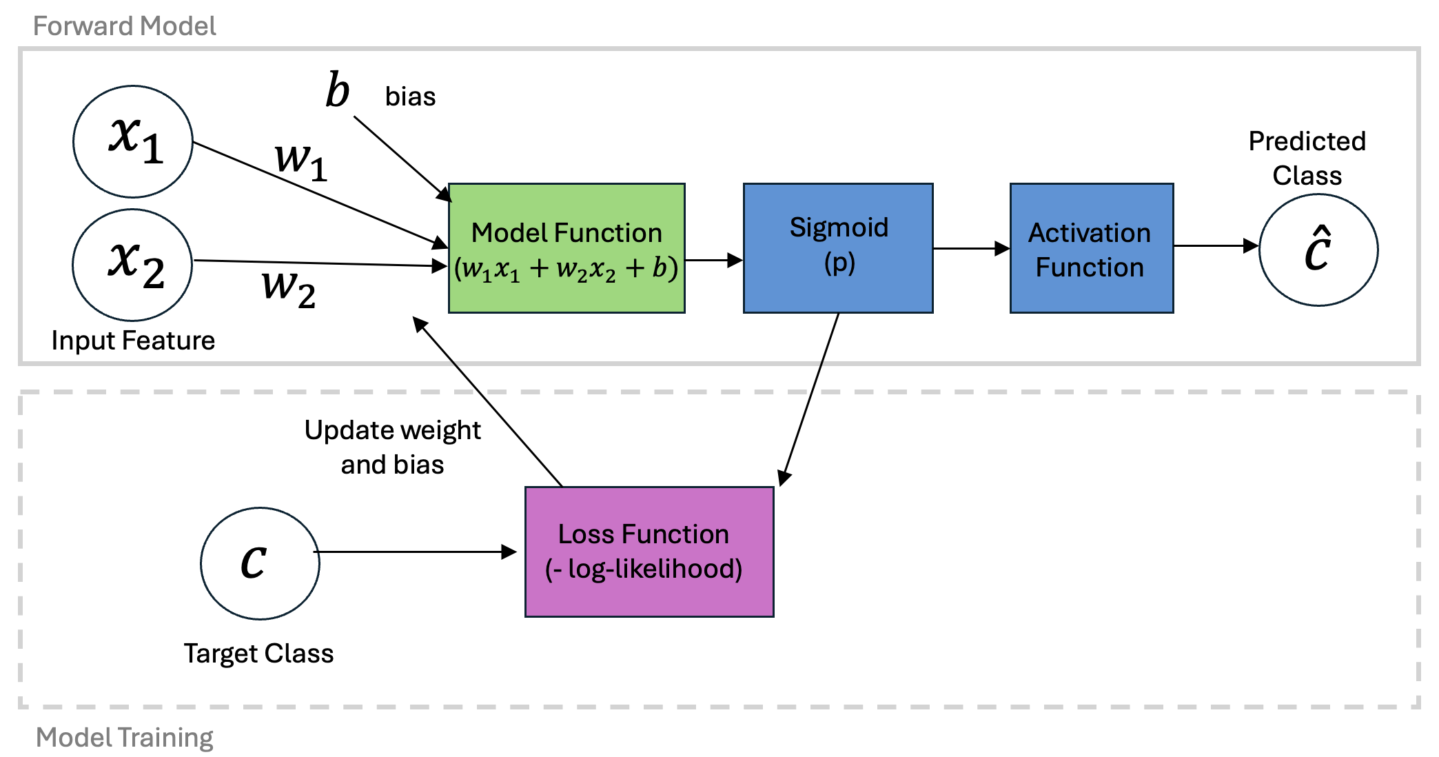
Given the commonalities with the previous models, we will see some strong parallels in the code:

class LogisticRegression:
    def __init__(self, X, learning_rate=0.001, n_iters=1000, random_seed=1):
        """
        Parameters:
        - X: Training data matrix (num_samples x num_features)
        - learning_rate: Step size for weight updates
        - n_iters: Number of training iterations
        - random_seed: Seed for reproducibility
        """
        self.lr = learning_rate
        self.n_iters = n_iters
        self.random_seed = random_seed
        self.initialize(X)
        
    def initialize(self, X):
        """
        Initializes the weight vector with small random values.
        """
        np.random.seed(self.random_seed)
        self.w = np.random.normal(loc=0.0, scale=0.01, size=np.shape(X)[1])

    def activation(self, x):
        """Binary step activation function"""
        return np.where(x >= 0.5, 1, 0)

    def sigmoid(self,x):
        """Sigmoid function to map values to range 0-1"""
        return 1 / (1 + np.exp(-x))

    def predict_probability(self, X):
        """Probability based on linear model and sigmoid transformation"""
        probability = self.sigmoid(np.dot(X, self.w))
        return probability

    def loss(self, p, c):
        """Log-liklihood function multiplied by -1"""
        loss = -np.sum(c * np.log(p + 1e-8) + (1 - c) * np.log(1 - p + 1e-8))
        return(loss)

    def fit(self, X, c):
        """Train the logistic regression model"""
        self.losses = []
        for iteration in range(self.n_iters):
            probability = self.predict_probability(X)
            p_c = np.array((probability-c)).reshape((len(c), 1))
            gradient = np.dot(p_c.T, X).ravel()
            self.w -= self.lr * gradient
            self.losses.append(self.loss(probability, c))
       
    def predict(self, X):
        """Predict binary labels for input data"""
        probability = self.predict_probability(X)
        return self.activation(probability).astype(int)

Let’s see how our model works in action! Let’s fit it to our normalized data:

X = np.column_stack([np.ones_like(df['SL_norm']), df['SL_norm'], df['CBL_norm']])
model = LogisticRegression(X,n_iters=1000)
model.fit(X,df['Classification'])

Next, let’s see how our model looks:

classifications_model = model.predict(X)

x1_data_span = np.linspace(min_x,max_x,500)
x2_data_span = np.linspace(min_y,max_y,500)
X1_data_span, X2_data_span = np.meshgrid(x1_data_span, x2_data_span)
P = model.predict_probability(np.column_stack([np.ones(np.size(X1_data_span),),
                                         X1_data_span.ravel(),
                                         X2_data_span.ravel()]))
P = P.reshape(np.shape(X1_data_span))

plt.figure(figsize=(11,4))

plt.subplot(1,2,1)
plt.plot(df['SL_norm'][classifications_model==0],
         df['CBL_norm'][classifications_model==0],'b.',label='Class 0 (Male)')
plt.plot(df['SL_norm'][classifications_model==1],
         df['CBL_norm'][classifications_model==1],'r.',label='Class 1 (Female)')
C = plt.pcolormesh(X1_data_span, X2_data_span, P, cmap='coolwarm', alpha=0.5)
plt.contour(X1_data_span, X2_data_span, P, levels=[0.5], colors='white')
plt.colorbar(C, label='Probability of Belonging to Class 1')
plt.gca().set_xlim([min_x,max_x])
plt.gca().set_ylim([min_y,max_y])
plt.legend(loc=2)
plt.title('Modeled Classifications')

plt.subplot(1,2,2)
plt.plot(model.losses)
plt.ylabel('Loss')
plt.xlabel('Iterations')

plt.show()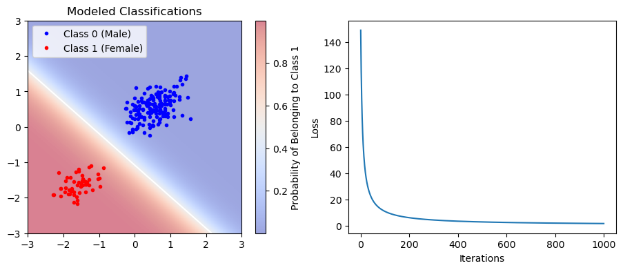

Using the Trained Logistic Regression Model¶

Ok, now that we’ve got our trained model (either the Logistic Regression model here or the previous Perceptron model), how do we use it? Well, we could imagine an independent measurement of a sea lion from our underwater photography as follows:

body_length = 240 #cm
skull_length = 260 #mm

To use this in our model, we need to first apply the standardization transformation:

body_length_norm = (body_length - np.mean(df['SL']))/(np.std(df['SL']))
skull_length_norm = (skull_length - np.mean(df['CBL']))/(np.std(df['CBL']))

Then, we pass these into the predict method using the expected vector format:

classification = model.predict([1,body_length_norm,skull_length_norm])

if classification==0:
    print('This sea lion is classified as male')
else:
    print('This sea lion is classified as female')

This sea lion is classified as male

Note that this only gives us the classification - but using our Logistic Regression model, we can also assign a probability to this classification. Let’s compute that here:

probability = model.predict_probability([1,body_length_norm,skull_length_norm])

Recall how we formulated our probability above - this is the probability that the sample belongs to class 1. In other words, it is the probability that the sea lion is female:

print(f'There is a {100*probability:.2f}% chance that this sea lion is female')

There is a 2.93% chance that this sea lion is female

Note that this probability feature is a key component of Logistic Regression model but not the Perception model.

Key Takeaways

Logistic regression assumes a linear relationship between the input features and the log-odds of a sample belonging to a given class
The model assigns not only a classification to a give class, but also a probability.
Despite the unique formulation of the problem, the structure of the class is very similar to the linear regression and perception classes.