In this notebook, we will get familiar with convolutional neural networks (CNNs) - an important neural network structure for image analysis.
Learning Objectives
Describe the convolution calculation and how it is applied to images.
Outline the components of a convolutional neural network.
Implement a convolutional neural network in PyTorch.
Import modules
Begin by importing the modules to be used in this notebook.
import os
import numpy as np
import matplotlib.pyplot as plt
import matplotlib.gridspec as gridspec
import scipy
from PIL import Image
# modules from PyTorch
import torch
import torch.nn as nn
import torch.optim as optim
from torchvision import datasets, transforms
from torch.utils.data import DataLoaderLet’s prepare our device to use PyTorch
if torch.cuda.is_available():
    device_name = "cuda"
elif torch.backends.mps.is_available():
    device_name = "mps"
else:
    device_name = "cpu"
print('Using device: '+device_name)
device = torch.device(device_name)
Using device: mps
Motivation
As beings with a visual cortex, images comprise a great deal of the information we receive and how we interact with the world. As a result, much of the data we use is stored as images.
As data, images are stored as two- or three-dimensional arrays with coherent spatial information. For example, consider the following image of a yellow sea sponge:
image = Image.open('../images/yellow_sponge.png').convert('RGB')
image_array = np.array(image)
plt.imshow(image)
plt.title('Image Shape: '+str(np.shape(image_array)))
plt.show()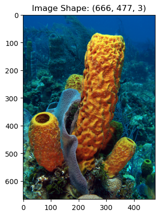
The above image is a yellow tube sponge (Aplysina fistularis). Image is courtesy of Wikimedia Commons. As we can see in this example, the image is a three-dimensional array with the dimensions corresponding to the shape of the image and the three “color bands” red, blue, and green. These bands are combined to produce the colors our human eyes can interpret.
This image is relatively small - just 666x477x3 pixels (in comparison to the 1000s of pixels in, say, modern cell phone camera images). But consider using one of the previous neural network architectures to examine a set of images like this to learn some desirable features. The previous architectures we looked at take in a one-dimensional vector. We might consider “unraveling” the images into a long one-dimensional vector as we did before, but this has two downsides:
This image would require 953,046 weights in each layer, which would be an incredibly expensive model to train and run.
More importantly, by “unraveling” the images, we lose all of the spatial information in the image. In other words, the neighboring points in an image are typically closely related and provide some information about each other.
In short, this approach would not only make our model very expensive, it would also remove valuable information from its construction. To solve this problem, we’ll need a relatively cheap two-dimensional operation that can be used to learn about the features in an image - it turns out that a convolution is just the thing we need.
Convolution
A convolution is a mathematical operation that involves an input matrix and a convolutional kernel. A convolution can be defined for vectors of any dimension but since the focus here is on CNNs that use 2-dimensional convolutions, the following examples will be shown in 2d.
Consider a matrix of size (3,3) and a convolutional kernel of size (3,3). The convolution of A with K is denoted as
When is a larger matrix, the convolution is achieved by “sliding” the kernel over the rows and columns of .
One step of this process can be visualized in the following diagram:
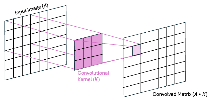
As we can see in the above image, the value of on row 1 and column 1 is the dot product of values of A in the upper-left 3x3 region of A with the values in the kernel K. This convolution process is then repeated by “sliding” the kernel across all of the rows and columns of to fill in the rest of the matrix.
A Concrete 2D Convolution Example: The Sobel filter
Convolutions have many uses for image processing and different kernels comprised of different organizations of weights have different purposes. Take, for example, the Sobel gradient filter - a simple edge detection filter. The Sobel filter works in two pieces - a gradient in the horizontal direction and a gradient in the vertical direction. Then the result of these two gradients is used to compute a magnitude, which can be thought of as the “sharpness” of the edge.
The kernels for the horizontal and vertical gradients are as follows:
These can be thought of as centered-difference approximation to the derivative in the and directions.
Let’s see how convolution with these kernels works on an example matrix:
# make the gradients
Kx = np.array([[-1, 0, 1], [-2, 0, 2], [-1, 0, 1]])
Ky = np.array([[-1, -2, -1], [0, 0, 0], [1, 2, 1]])
# make a test matrix
A = np.array([[1, 2, 3], [4, 5, 6], [7, 8, 9]])# compute the convolution using scipy
scipy.signal.convolve2d(A, Kx, mode='valid')array([[-8]])We get this result because
Hmm, but wait - what about the minus sign? In practice, deep learning libraries implement cross-correlation but refer to it as convolution. The calculations are identical, but the difference is that the kernel is “flipped” in a convolution while it is not flipped in a cross-correlation. Check this out:
# compute the correlation using scipy
scipy.signal.correlate(A, Kx, mode='valid')array([[8]])Let’s see how convolution works by applying this filter to our sponge image. We can use these kernels across the image to compute the edges. Let’s first convert this image to grayscale to keep things a little more clear:
image=image.convert('L')
image_array = (np.array(image)-255)/255
Next, we can compute the convolution:
# make empty arrays for the convolution
Gx = np.zeros_like(image_array)
Gy = np.zeros_like(image_array)

# loop through the rows and columns of the image to
# compute the convolution of the image and the kernel
for row in range(1,np.shape(Gx)[0]-1):
    for col in range(1,np.shape(Gy)[1]-1):
        Gx[row,col] = scipy.signal.correlate(image_array[row-1:row+2, col-1:col+2],
                                              Kx, mode='valid')[0][0]
        Gy[row,col] = scipy.signal.correlate(image_array[row-1:row+2, col-1:col+2],
                                              Ky, mode='valid')[0][0]
Let’s make a quick plot and see what our gradients look like:
plt.figure(figsize=(12,5))
plt.subplot(1,4,1)
plt.imshow(Gx, cmap='Grays_r')
plt.title('Horizontal Gradient')
plt.axis('off')

plt.subplot(1,4,2)
plt.imshow(Gy, cmap='Grays_r')
plt.title('Vertical Gradient')
plt.axis('off')

plt.subplot(1,4,3)
plt.imshow((Gx**2 + Gy**2)**0.5, cmap='Grays_r')
plt.title('Gradient Magnitude')
plt.axis('off')

plt.subplot(1,4,4)
plt.imshow(image_array, cmap='Grays_r')
plt.title('Grayscale Image')
plt.axis('off')

plt.tight_layout()
plt.show()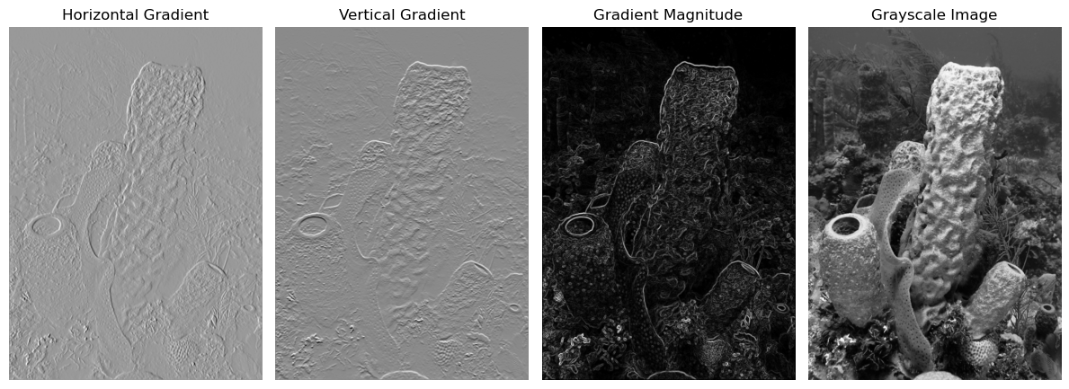
Our First CNN
Now that we’re familiar with the idea of a convolution, let’s see how we can leverage this operation for image classification.
A Peek at the Data
In this example, we will use a set of images for sea creatures that have been classified into five categories - one for each creature. The data are stored into a directory called “Images” with subdirectories for training, testing, and validation. Within each subdirectory, there are additional subdirectories for each of the five classifications [0-4]. Each image has a width and height of 100 pixels each, and there are three “channels” in the image for the red, green, and blue colors that constitute the image.
Let’s take a look at the first image of each species in the training data:
# define the species for each category
species = ['sea sponge','sea star','crab','plankton','squid']

# make a figure object
fig = plt.figure(figsize=(10,3))
gs = gridspec.GridSpec(1,5)

# plot the first image for each of the species from the training dataset
for s in range(len(species)):

    # load image
    image_list = os.listdir(os.path.join('..','data','sea_creature_images','train',str(s)))
    image = Image.open(os.path.join('..','data','sea_creature_images','train',str(s),image_list[0])).convert('RGB')

    # plot the image on an axis
    ax = fig.add_subplot(gs[0, s])
    ax.imshow(image)
    ax.axis('off')
    ax.set_title(species[s])

plt.suptitle('True Labels of Images in the Training Set')
plt.show()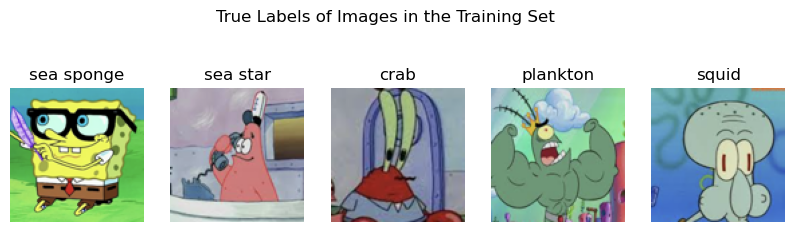
Defining the CNN Architecture
In this example, we will begin with a relatively simple CNN architecture - one that has two convolutional layers, each with an activation function and a pooling layer, and two additional fully-connected layers. Visually, we can represent this architecture graphically as follows:
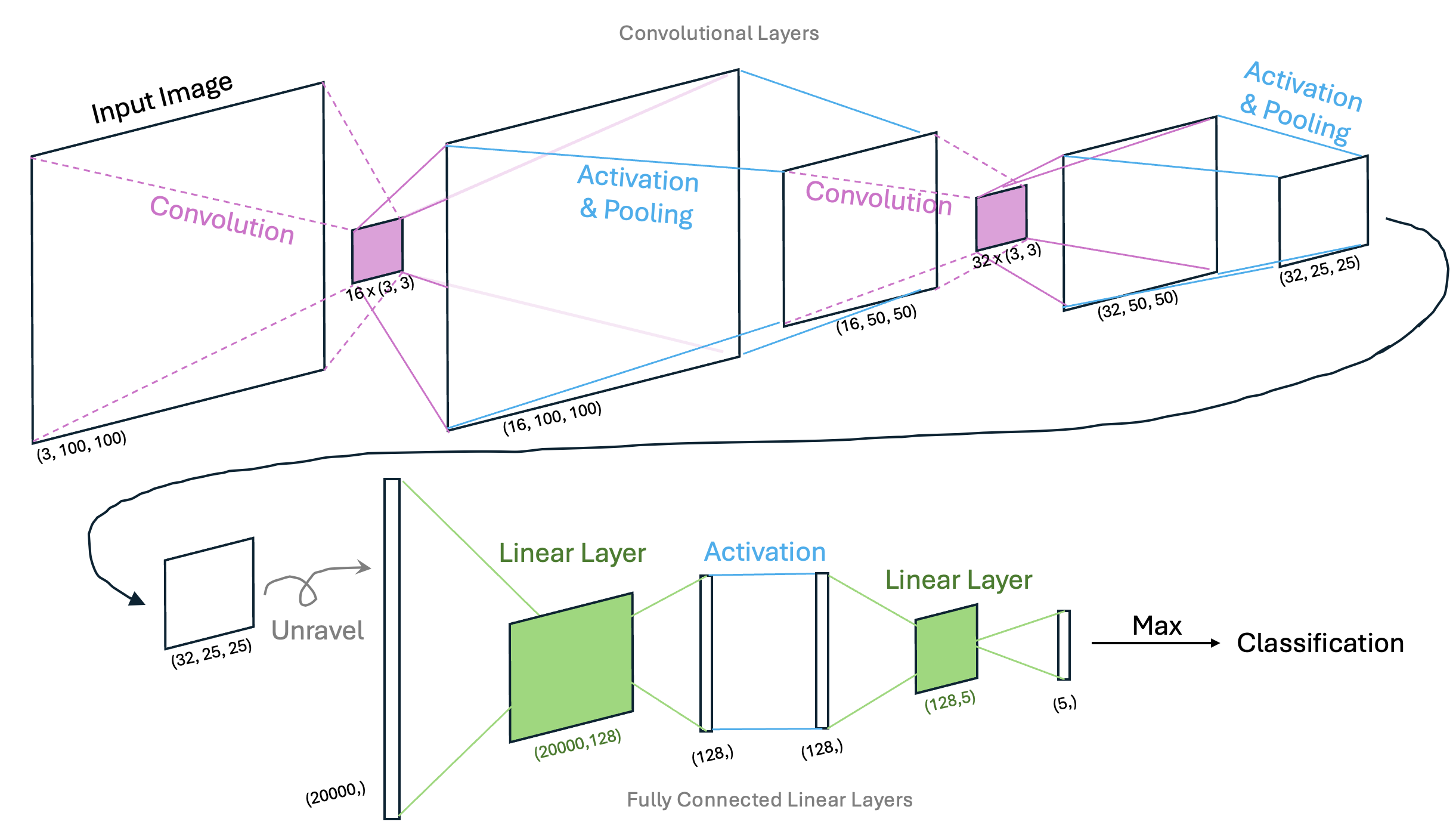
In this example, the first two convolutional layers are used to extract pertinent features in the images that may pertain to each species of sea creature. For example, sea sponges may be defined by straight edges or corners while sea stars may be defined by triangular features. The pooling layers allow us to sample patterns in the images at different scales. Finally, the fully connected layers provide a mechanism to classify the images based on the prominent patterns for each species. When examining this network, it’s important to be able to identify what is being trained so we’ll state this explicitly: in a CNN, weights in both the convolutional kernels and the linear layers are optimized via back propagation and gradient descent.
Using PyTorch, we can construct a class for this CNN as follows:
class ClassificationCNN(nn.Module):
    def __init__(self):
        super(ClassificationCNN, self).__init__()

        # construct the convolutional layers
        self.conv_layers = nn.Sequential(
            nn.Conv2d(3, 16, kernel_size=3, padding=1),  # output shape: (16, 100, 100)
            nn.ReLU(),
            nn.MaxPool2d(2),  # output shape: (16, 50, 50)

            nn.Conv2d(16, 32, kernel_size=3, padding=1),  # output shape: (32, 50, 50)
            nn.ReLU(),
            nn.MaxPool2d(2)   # output shape: (32, 25, 25)
        )

        # construct the fully connected layers
        conv_output_size = 32 * (25) * (25)
        self.fc_layers = nn.Sequential(
            nn.Flatten(), # output shape: (20000,)
            nn.Linear(conv_output_size, 128), # output shape: (128,)
            nn.ReLU(),
            nn.Linear(128, 5) # output shape: (5,)
        )

    # define the forward step
    def forward(self, x):
        x = self.conv_layers(x)
        x = self.fc_layers(x)
        return x
New Layers
In the class above, we see three different layers we haven’t encountered in previous networks
nn.Conv2d(3, 16, kernel_size=3, padding=1)- this layer implements the 2D convolutional layer, In this case, we implement a set of 16 3x3x3 kernels. Since each kernel is applied to the input image, the number of channels will increase from 3 to 16 in the subsequent step of the network.nn.ReLU()- ReLU is short for “Rectified Linear Unit” and is another activation function similar to the sigmoid activation function we’ve seen previously. The ReLU activation function returns 0 for negative value and is the identity function for positive values. This is a common choice for neural networks with many layers.nn.MaxPool2d(2)- max pooling layer chooses the most prominent features in a given area of a pixel. In this case, the maximum value from each 2x2 layer is passed to the next layer and the dimensions of the image will reduce by half.
Preprocessing the input data
In addition to the architecture of the CNN itself, we also need to identify how we will preprocess the images before feeding them into the network. Here, we will transform the images to PyTorch tensors, and then normalize the data:
transform = transforms.Compose([
    transforms.ToTensor(),
    transforms.Normalize(mean=[0.5, 0.5, 0.5], std=[0.5, 0.5, 0.5])  # 3 values for RGB
])
Using the Model
Now that we’ve defined the model, we can use it to classify images. For example, we could use the model to test the first image in the validation dataset for each species:
# define the model
model = ClassificationCNN().to(device)

# put the model in evaluation mode
model.eval()

# make a figure object
fig = plt.figure(figsize=(10,3))
gs = gridspec.GridSpec(1,5)

# plot the classifications of the first image for each of the species from the testing dataset
for s in range(len(species)):

    # load image
    image_list = os.listdir(os.path.join('..','data','sea_creature_images','validate',str(s)))
    image = Image.open(os.path.join('..','data','sea_creature_images','validate',str(s),image_list[0])).convert('RGB')

    # get the prediction of the species
    input_tensor = transform(image).unsqueeze(0).to(device)
    with torch.no_grad():
        output = model(input_tensor)
        _, predicted = torch.max(output, 1)
    predicted_species = species[predicted.item()]

    # plot the image on an axis
    ax = fig.add_subplot(gs[0, s])
    ax.imshow(image)
    ax.axis('off')
    ax.set_title(predicted_species)

plt.suptitle('Predicted Labels of Images in the Validation Dataset before Training')
plt.show()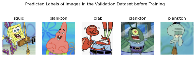
As we can see, the model isn’t doing well - and that’s to be expected since we haven’t done any training to optimize the weights in the convolutional kernels or the fully connected layers. Let’s go ahead and do that now.
Run a Training Loop
To run a training loop, first we will leverage a few tools to load in the training and testing data:
# define the training and testing mechanisms to load in images as datasets
BATCH_SIZE = 10

# first construct the training set
train_dataset = datasets.ImageFolder(root=os.path.join('..','data','sea_creature_images','train'), transform=transform)
train_loader = DataLoader(train_dataset, batch_size=BATCH_SIZE, shuffle=True)

# then the testing set
test_dataset = datasets.ImageFolder(root=os.path.join('..','data','sea_creature_images','test'), transform=transform)
test_loader = DataLoader(test_dataset, batch_size=BATCH_SIZE, shuffle=False)
Next, let’s define the loss function and the gradient descent function. Since this is a classification example, we will use the Cross Entropy Loss function:
# cross entropy loss for use in classification problems
criterion = nn.CrossEntropyLoss()
The cross entropy loss function is common for classification tasks and is defined as follows:
Intuitively, we can see that, for a given training example, the probabilities will be zero for each class except for the one with the true label (since they are one-hot encoded). When , the loss will be very large when is close to zero (due to the minus sign in front), and then loss will be small when is close to 1.
For comparison, we can see this is similar to the MSE loss function we used in our single- and multi-layer perceptrons.
We are nearly ready to run our training loop but first, let’s bundle up a function to compute the number of correct labels in a set of output so that we can report stats in our training example:
def compute_correct_labels(outputs, labels):
    correct = 0
    total = 0
    _, predicted_values = torch.max(outputs, 1)
    differences = predicted_values - labels
    for i in range(len(differences)):
        if differences[i]==0:
            correct +=1
        total += 1
    return(correct, total)
Finally, we are ready to run our training loop. To alleviate duplicating code in this notebook, let’s write this up into a training loop function:
def training_loop(model, optimizer, NUM_EPOCHS, train_loader, test_loader, printing=True):
    # make empty lists to keep track of the training and testing losses
    train_losses = []
    test_losses = []

    # loop through each epoch to run the training loop
    # and check the model with the training data
    # keep track of both sets of losses as you go
    for epoch in range(NUM_EPOCHS):

        # Run the training loop
        model.train()
        total_train_loss = 0.0
        total_train_correct = 0
        total_train_images = 0
        for train_inputs, train_labels in train_loader:
            train_inputs, train_labels = train_inputs.to(device), train_labels.to(device)
            optimizer.zero_grad()
            outputs = model(train_inputs)
            train_correct, train_total = compute_correct_labels(outputs, train_labels)
            total_train_correct += train_correct
            total_train_images += train_total
            loss = criterion(outputs, train_labels)
            loss.backward()
            optimizer.step()
            total_train_loss += loss.item()
        avg_train_loss = total_train_loss / len(train_loader)
        train_losses.append(avg_train_loss)

        # Run the testing loop
        # this is essentially the same as the training loop but
        # without the optimizer and backward propagation
        model.eval()
        total_test_loss = 0.0
        total_test_correct = 0
        total_test_images = 0
        with torch.no_grad():
            for test_inputs, test_labels in test_loader:
                test_inputs, test_labels = test_inputs.to(device), test_labels.to(device)
                outputs = model(test_inputs)
                test_correct, test_total = compute_correct_labels(outputs, test_labels)
                total_test_correct += test_correct
                total_test_images += test_total
                loss = criterion(outputs, test_labels)
                total_test_loss += loss.item()
        avg_test_loss = total_test_loss / len(test_loader)
        test_losses.append(avg_test_loss)

        if printing:
            print(f"Epoch {epoch+1}/{NUM_EPOCHS}"+\
                  f" - Train Loss: {avg_train_loss:.4f}, "+\
                  f"Train Correct: {total_train_correct}/{total_train_images} "+\
                  f"- Test Loss: {avg_test_loss:.4f}, "+\
                  f"Test Correct: {total_test_correct}/{total_test_images} ")

    return(train_losses, test_losses)
# redefine the model here in case cells are run out of order
# for instructional purposes
model = ClassificationCNN().to(device)
# Adam optimizer for stochastic gradient descent
# note that this uses the given model object's parameters
# and therefore must be defined after the model is defined
optimizer = optim.Adam(model.parameters(), lr=0.001)
# define the number of epochs
NUM_EPOCHS = 20
# run the training loop function
train_losses, test_losses = training_loop(model, optimizer, NUM_EPOCHS, train_loader, test_loader)Epoch 1/20 - Train Loss: 1.5771, Train Correct: 63/175 - Test Loss: 1.4025, Test Correct: 20/50
Epoch 2/20 - Train Loss: 1.0244, Train Correct: 120/175 - Test Loss: 1.4411, Test Correct: 18/50
Epoch 3/20 - Train Loss: 0.6342, Train Correct: 130/175 - Test Loss: 2.2425, Test Correct: 17/50
Epoch 4/20 - Train Loss: 0.4495, Train Correct: 144/175 - Test Loss: 1.1854, Test Correct: 30/50
Epoch 5/20 - Train Loss: 0.1899, Train Correct: 165/175 - Test Loss: 1.1741, Test Correct: 32/50
Epoch 6/20 - Train Loss: 0.0727, Train Correct: 173/175 - Test Loss: 0.7389, Test Correct: 34/50
Epoch 7/20 - Train Loss: 0.0320, Train Correct: 175/175 - Test Loss: 1.0786, Test Correct: 30/50
Epoch 8/20 - Train Loss: 0.0191, Train Correct: 175/175 - Test Loss: 0.9870, Test Correct: 39/50
Epoch 9/20 - Train Loss: 0.0071, Train Correct: 175/175 - Test Loss: 0.8829, Test Correct: 39/50
Epoch 10/20 - Train Loss: 0.0047, Train Correct: 175/175 - Test Loss: 0.9653, Test Correct: 38/50
Epoch 11/20 - Train Loss: 0.0032, Train Correct: 175/175 - Test Loss: 0.9380, Test Correct: 39/50
Epoch 12/20 - Train Loss: 0.0024, Train Correct: 175/175 - Test Loss: 0.9474, Test Correct: 39/50
Epoch 13/20 - Train Loss: 0.0020, Train Correct: 175/175 - Test Loss: 0.9517, Test Correct: 39/50
Epoch 14/20 - Train Loss: 0.0018, Train Correct: 175/175 - Test Loss: 0.9853, Test Correct: 39/50
Epoch 15/20 - Train Loss: 0.0014, Train Correct: 175/175 - Test Loss: 0.9756, Test Correct: 38/50
Epoch 16/20 - Train Loss: 0.0012, Train Correct: 175/175 - Test Loss: 1.0006, Test Correct: 39/50
Epoch 17/20 - Train Loss: 0.0011, Train Correct: 175/175 - Test Loss: 1.0139, Test Correct: 39/50
Epoch 18/20 - Train Loss: 0.0010, Train Correct: 175/175 - Test Loss: 1.0218, Test Correct: 39/50
Epoch 19/20 - Train Loss: 0.0009, Train Correct: 175/175 - Test Loss: 1.0309, Test Correct: 39/50
Epoch 20/20 - Train Loss: 0.0008, Train Correct: 175/175 - Test Loss: 1.0353, Test Correct: 38/50
The Adaptive Moment Estimation Algorithm
In the training loop function above, you may have noticed we used the following algorithm as our optimizer: optim.Adam(model.parameters(), lr=0.001)
Here, Adam (short for Adaptive Moment Estimation) is a gradient descent algorithm much like the (Stochastic) Gradient Descent algorithm (SGD) we’ve used in previous lessons. The difference here is that the Adam algorithm chooses updates to weights in a “smarter way” than randomly taking steps toward the minimum of the loss function. This is done by computing the running mean and the variance of the gradients as they are computed on each iteration. These quantities (or “moments”) are used to scale the learning rate so that the steps are appropriately sized - e.g. large steps are taken when possible, but small steps are used when there may be an issue of convergence. This is a popular choice for learning algorithms and we will use it in most of the subsequent examples.
Visualize the Training and Testing Losses
Now that we’ve run our training loop, let’s have a peek at our training and testing losses. This should give us a sense for how well our model is doing and what issues might be hiding in our design:
plt.figure(figsize=(8, 4))
plt.plot(range(1, NUM_EPOCHS + 1), train_losses, 'd-', label='Training Loss')
plt.plot(range(1, NUM_EPOCHS + 1), test_losses, 'd-', label='Test Loss')
plt.xlabel('Epoch')
plt.ylabel('Loss')
plt.title('Training and Testing Loss Over Epochs')
plt.legend()
plt.grid(True)
plt.tight_layout()
plt.show()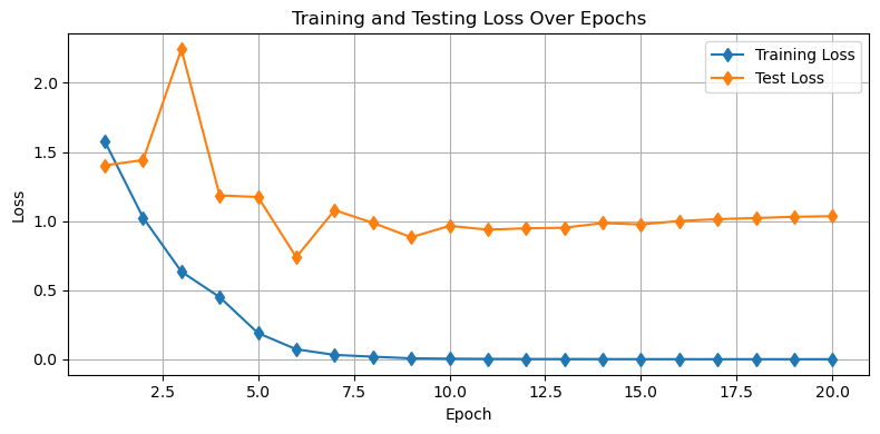
Questions for Consideration
How is the model performing on the training data?
How is the model performing on the testing data?
To what extent might this model be underfit or overfit?
Test the Model on the Validation Set
We can see in the plot above that there are likely some issues in our model. Don’t worry - we will address that next. For now, let’s see how our model is doing on each of the images in our validation set.
First, define an image loader just like we did for our training and testing data:
validation_dataset = datasets.ImageFolder(root=os.path.join('..','data','sea_creature_images','validate'), transform=transform)
validation_loader = DataLoader(validation_dataset, batch_size=5, shuffle=False)
Next, let’s apply the model to each of our 5 validation images for each of the 5 species:
# Set model to evaluation mode
model.eval()

# make a figure object
fig = plt.figure(figsize=(9,9))
gs = gridspec.GridSpec(5, len(species))

# loop through each species (column)
for s in range(len(species)):

    # loop through the image files
    file_list = os.listdir(os.path.join('..','data','sea_creature_images','validate',str(s)))[:5]
    for file_count, file_name in enumerate(file_list):

        # load the image
        image = Image.open(os.path.join('..','data','sea_creature_images','validate',str(s),file_name)).convert('RGB')
        input_tensor = transform(image).unsqueeze(0).to(device)  # Add batch dimension

        # get the predicted class
        with torch.no_grad():
            output = model(input_tensor)
            _, predicted = torch.max(output, 1)
        predicted_class = species[predicted.item()]

        # add the image to the plot with the prediction
        ax = fig.add_subplot(gs[file_count, s])
        ax.imshow(image)
        ax.axis('off')
        ax.set_title(predicted_class)
        file_count +=1

plt.suptitle('Predicted Labels of All Images in the Validation Dataset after Training')
plt.show()
Our model is working pretty well on the validation set! However, there’s still lots of room for improvement here. Let’s see what our options are in the next notebook.
Improving the Performance of Convolutional Neural Networks
In our previous example, we built a convolutional neural network for image classification but we found that our model was too complex for our data - and the model “memorized” the dataset. In this notebook, we will explore two methods that can help alleviate overfitting.
Dropout
Dropout refers to the process of “dropping out” certain nodes in the network at random by setting their weights to 0 in one pass through the forward model. You’ll recall that our linear layers are implemented with fully-connected nodes meaning all input features to a layer are connected to all output nodes via an individual weight. Dropping out is typically done on the fully-connected layers in a CNN but it may also be done in the convolutional layers.
Since this technique is quite common, it is built into the nn module of PyTorch and we can slip this into our CNN:
class ClassificationCNN(nn.Module):
    def __init__(self):
        super(ClassificationCNN, self).__init__()

        self.conv_layers = nn.Sequential(
            nn.Conv2d(3, 16, kernel_size=3, padding=1),
            nn.ReLU(),
            nn.MaxPool2d(2),
            nn.Conv2d(16, 32, kernel_size=3, padding=1),
            nn.ReLU(),
            nn.MaxPool2d(2)
        )

        conv_output_size = 32 * (25) * (25)
        self.fc_layers = nn.Sequential(
            nn.Flatten(),
            nn.Linear(conv_output_size, 128),
            nn.ReLU(),
            nn.Dropout(p=0.8), # NEW! Drop out some of the 128 nodes at random
                               # with an 80% probability
            nn.Linear(128, 5)
        )

    # define the forward step
    def forward(self, x):
        x = self.conv_layers(x)
        x = self.fc_layers(x)
        return x
With this change, we can proceed to training our model using our training function:
# redefine the model here in case cells are run out of order
# for instructional purposes
model = ClassificationCNN().to(device)

# Adam optimizer for stochastic gradient descent
optimizer = optim.Adam(model.parameters(), lr=0.001)

# define the number of epochs
NUM_EPOCHS = 20

# call the training loop function we defined above
train_losses, test_losses = training_loop(model, optimizer, NUM_EPOCHS,
                                          train_loader, test_loader)
Epoch 1/20 - Train Loss: 1.8580, Train Correct: 37/175 - Test Loss: 1.5948, Test Correct: 17/50
Epoch 2/20 - Train Loss: 1.5826, Train Correct: 55/175 - Test Loss: 1.5644, Test Correct: 13/50
Epoch 3/20 - Train Loss: 1.5664, Train Correct: 42/175 - Test Loss: 1.4810, Test Correct: 21/50
Epoch 4/20 - Train Loss: 1.4476, Train Correct: 70/175 - Test Loss: 1.3953, Test Correct: 19/50
Epoch 5/20 - Train Loss: 1.3984, Train Correct: 68/175 - Test Loss: 1.3229, Test Correct: 22/50
Epoch 6/20 - Train Loss: 1.2164, Train Correct: 86/175 - Test Loss: 1.3090, Test Correct: 26/50
Epoch 7/20 - Train Loss: 1.2005, Train Correct: 76/175 - Test Loss: 1.1844, Test Correct: 28/50
Epoch 8/20 - Train Loss: 1.0913, Train Correct: 89/175 - Test Loss: 1.2161, Test Correct: 30/50
Epoch 9/20 - Train Loss: 1.0214, Train Correct: 101/175 - Test Loss: 1.0363, Test Correct: 30/50
Epoch 10/20 - Train Loss: 0.9682, Train Correct: 98/175 - Test Loss: 1.0504, Test Correct: 29/50
Epoch 11/20 - Train Loss: 0.9381, Train Correct: 111/175 - Test Loss: 0.9877, Test Correct: 31/50
Epoch 12/20 - Train Loss: 0.8757, Train Correct: 118/175 - Test Loss: 1.0923, Test Correct: 33/50
Epoch 13/20 - Train Loss: 0.7144, Train Correct: 127/175 - Test Loss: 0.9341, Test Correct: 32/50
Epoch 14/20 - Train Loss: 0.6875, Train Correct: 125/175 - Test Loss: 1.0419, Test Correct: 29/50
Epoch 15/20 - Train Loss: 0.6866, Train Correct: 125/175 - Test Loss: 0.9061, Test Correct: 36/50
Epoch 16/20 - Train Loss: 0.6924, Train Correct: 119/175 - Test Loss: 0.7767, Test Correct: 35/50
Epoch 17/20 - Train Loss: 0.6355, Train Correct: 137/175 - Test Loss: 1.2683, Test Correct: 27/50
Epoch 18/20 - Train Loss: 0.6889, Train Correct: 136/175 - Test Loss: 0.9040, Test Correct: 33/50
Epoch 19/20 - Train Loss: 0.5909, Train Correct: 137/175 - Test Loss: 0.9252, Test Correct: 35/50
Epoch 20/20 - Train Loss: 0.5302, Train Correct: 134/175 - Test Loss: 0.8761, Test Correct: 30/50
plt.figure(figsize=(8, 4))
plt.plot(range(1, NUM_EPOCHS + 1), train_losses, 'd-', label='Training Loss')
plt.plot(range(1, NUM_EPOCHS + 1), test_losses, 'd-', label='Test Loss')
plt.xlabel('Epoch')
plt.ylabel('Loss')
plt.title('Training and Testing Loss Over Epochs')
plt.legend()
plt.grid(True)
plt.tight_layout()
plt.show()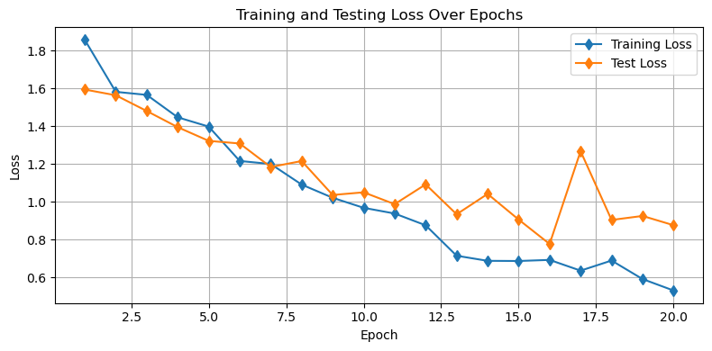
Looking at the plot above, we can see that the dropout procedure helped with our issue of overfitting! Now, we don’t see an increase in the test losses as the training is declining - both decline at the same rate.
A peek at model performance on the validation set
Let’s take a peek at how things are looking in our validation set:
# define the species for each category
species = ['sea sponge','sea star','crab','plankton','squid']

# Set model to evaluation mode
model.eval()

# make a figure object
fig = plt.figure(figsize=(9,9))
gs = gridspec.GridSpec(5, len(species))

# loop through each species (column)
for s in range(len(species)):

    # loop through the image files
    file_list = os.listdir(os.path.join('..','data','sea_creature_images','validate',str(s)))[:5]
    for file_count, file_name in enumerate(file_list):

        # load the image
        image = Image.open(os.path.join('..','data','sea_creature_images','validate',str(s),file_name)).convert('RGB')
        input_tensor = transform(image).unsqueeze(0).to(device)  # Add batch dimension

        # get the predicted class
        with torch.no_grad():
            output = model(input_tensor)
            _, predicted = torch.max(output, 1)
        predicted_class = species[predicted.item()]

        # add the image to the plot with the prediction
        ax = fig.add_subplot(gs[file_count, s])
        ax.imshow(image)
        ax.axis('off')
        ax.set_title(predicted_class)
        file_count +=1

plt.suptitle('Predicted Labels of All Images in the Validation Dataset after Training')
plt.show()
Looks pretty good - let’s explore one other way we can improve our model to avoid overfitting.
Data Augmentation
Data augmentation is the process of supplementing the training data set to include more training examples when the training examples do not exist. To create these artificial training examples, we will apply transformations to our existing set in such a way that the character of the image remains intact while the actual pixel values have changed.
Since this augmentation procedure is quite common, the torchvision module is designed to give us a way to call upon typical transformations. Let’s have a look at a few of them:
# read the last image from the validation set
image = Image.open(os.path.join('..','data','sea_creature_images','validate',str(s),file_name)).convert('RGB')
input_tensor = transform(image).unsqueeze(0).to(device)  # Add batch dimension

# define a list of augmentations
augmentations = [transforms.ColorJitter(brightness=0.3, contrast=0.3, saturation=0.3, hue=0.05),
                 transforms.RandomPerspective(distortion_scale=0.4, p=1.0),
                 transforms.RandomHorizontalFlip(p=1.0),
                 transforms.RandomVerticalFlip(p=1.0),
                 transforms.RandomRotation(degrees=180)]
augmentation_names = ['ColorJitter','RandomPerspective','RandomHorizontalFlip',
                      'RandomVerticalFlip','RandomRotation']

# make a figure object
fig = plt.figure(figsize=(9,6))
gs = gridspec.GridSpec(2, 3)

# organize the plots of each image
ax = fig.add_subplot(gs[0,0])
ax.imshow(image)
ax.axis('off')
ax.set_title('Original Image')

for a, augmentation in enumerate(augmentations):
    transformed_image = augmentation(image)
    col = (a+1)%3
    row = (a+1)//3
    ax = fig.add_subplot(gs[(a+1)//3, (a+1)%3])
    ax.imshow(transformed_image)
    ax.axis('off')
    ax.set_title(augmentation_names[a])

plt.show()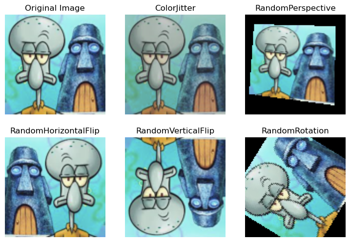
Data augmentation can be used to build up more images in the training set, stored as additional files. Alternatively, we can build these random transformations directly into our data loader so that each time we load up a mini-batch, the images are modified before being passed through the network.
Here, we will build in these transformations at random as the images are read in to PyTorch:
# training transform
train_transform_augmented = transforms.Compose([

    # Apply some random flips and rotations
    transforms.RandomHorizontalFlip(p=0.5), # 50% chance to apply this
    transforms.RandomVerticalFlip(p=0.5), # 50% chance to apply this
    transforms.RandomRotation(degrees=15),

    # Randomly apply one of these transformations
    transforms.RandomApply([
        transforms.ColorJitter(brightness=0.3, contrast=0.3, saturation=0.3, hue=0.05),
        transforms.RandomPerspective(distortion_scale=0.4, p=1.0)
    ], p=0.5),  # 50% chance to apply one of these

    transforms.ToTensor(),
    transforms.Normalize(mean=[0.5, 0.5, 0.5], std=[0.5, 0.5, 0.5])
])
Now that we’ve redefined our transform, let’s redefine our data loader:
# first construct the training set
train_dataset_augmented = datasets.ImageFolder(root=os.path.join('..','data','sea_creature_images','train'),
                                               transform=train_transform_augmented)
train_loader_augmented = DataLoader(train_dataset_augmented, batch_size=BATCH_SIZE, shuffle=True)
Let’s try our model with the new augmentation:
# redefine the model here in case cells are run out of order
# for instructional purposes
model = ClassificationCNN().to(device)

# Adam optimizer for stochastic gradient descent
optimizer = optim.Adam(model.parameters(), lr=0.001)

# define the number of epochs
NUM_EPOCHS = 30

# call the training loop function we defined above
train_losses, test_losses = training_loop(model, optimizer, NUM_EPOCHS,
                                        train_loader_augmented, test_loader)
Epoch 1/30 - Train Loss: 1.7967, Train Correct: 33/175 - Test Loss: 1.6081, Test Correct: 10/50
Epoch 2/30 - Train Loss: 1.6011, Train Correct: 43/175 - Test Loss: 1.5795, Test Correct: 17/50
Epoch 3/30 - Train Loss: 1.5607, Train Correct: 54/175 - Test Loss: 1.4904, Test Correct: 22/50
Epoch 4/30 - Train Loss: 1.5045, Train Correct: 65/175 - Test Loss: 1.3730, Test Correct: 26/50
Epoch 5/30 - Train Loss: 1.4221, Train Correct: 71/175 - Test Loss: 1.2275, Test Correct: 25/50
Epoch 6/30 - Train Loss: 1.3610, Train Correct: 71/175 - Test Loss: 1.1856, Test Correct: 25/50
Epoch 7/30 - Train Loss: 1.3043, Train Correct: 74/175 - Test Loss: 1.1322, Test Correct: 25/50
Epoch 8/30 - Train Loss: 1.2394, Train Correct: 87/175 - Test Loss: 1.1088, Test Correct: 27/50
Epoch 9/30 - Train Loss: 1.2681, Train Correct: 90/175 - Test Loss: 1.0357, Test Correct: 30/50
Epoch 10/30 - Train Loss: 1.1721, Train Correct: 94/175 - Test Loss: 1.0014, Test Correct: 34/50
Epoch 11/30 - Train Loss: 1.2541, Train Correct: 87/175 - Test Loss: 1.0027, Test Correct: 33/50
Epoch 12/30 - Train Loss: 1.1671, Train Correct: 85/175 - Test Loss: 1.0018, Test Correct: 32/50
Epoch 13/30 - Train Loss: 1.1563, Train Correct: 80/175 - Test Loss: 0.9297, Test Correct: 32/50
Epoch 14/30 - Train Loss: 1.0890, Train Correct: 103/175 - Test Loss: 0.8540, Test Correct: 40/50
Epoch 15/30 - Train Loss: 1.1180, Train Correct: 96/175 - Test Loss: 0.9965, Test Correct: 30/50
Epoch 16/30 - Train Loss: 1.1539, Train Correct: 95/175 - Test Loss: 0.9049, Test Correct: 37/50
Epoch 17/30 - Train Loss: 1.0409, Train Correct: 97/175 - Test Loss: 0.8738, Test Correct: 36/50
Epoch 18/30 - Train Loss: 0.9873, Train Correct: 102/175 - Test Loss: 0.8371, Test Correct: 37/50
Epoch 19/30 - Train Loss: 0.9740, Train Correct: 109/175 - Test Loss: 0.8398, Test Correct: 33/50
Epoch 20/30 - Train Loss: 0.9305, Train Correct: 110/175 - Test Loss: 0.8490, Test Correct: 37/50
Epoch 21/30 - Train Loss: 0.8880, Train Correct: 114/175 - Test Loss: 0.7393, Test Correct: 38/50
Epoch 22/30 - Train Loss: 0.9162, Train Correct: 106/175 - Test Loss: 0.7236, Test Correct: 38/50
Epoch 23/30 - Train Loss: 0.9710, Train Correct: 105/175 - Test Loss: 0.6861, Test Correct: 39/50
Epoch 24/30 - Train Loss: 0.9616, Train Correct: 113/175 - Test Loss: 0.6870, Test Correct: 39/50
Epoch 25/30 - Train Loss: 0.8586, Train Correct: 116/175 - Test Loss: 0.6421, Test Correct: 41/50
Epoch 26/30 - Train Loss: 0.8529, Train Correct: 120/175 - Test Loss: 0.6299, Test Correct: 41/50
Epoch 27/30 - Train Loss: 0.9232, Train Correct: 113/175 - Test Loss: 0.6764, Test Correct: 39/50
Epoch 28/30 - Train Loss: 0.9293, Train Correct: 110/175 - Test Loss: 0.6275, Test Correct: 38/50
Epoch 29/30 - Train Loss: 0.7826, Train Correct: 126/175 - Test Loss: 0.5949, Test Correct: 41/50
Epoch 30/30 - Train Loss: 0.7929, Train Correct: 122/175 - Test Loss: 0.6373, Test Correct: 39/50
plt.figure(figsize=(8, 4))
plt.plot(range(1, NUM_EPOCHS + 1), train_losses, 'd-', label='Training Loss')
plt.plot(range(1, NUM_EPOCHS + 1), test_losses, 'd-', label='Test Loss')
plt.xlabel('Epoch')
plt.ylabel('Loss')
plt.title('Training and Testing Loss Over Epochs')
plt.legend()
plt.grid(True)
plt.tight_layout()
plt.show()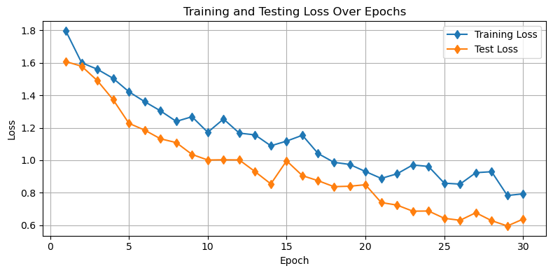
As we can see, the augmentation also helps yield training which avoids overfitting.
As above, we can check on the performance of our model on the validation set.
# define the species for each category
species = ['sea sponge','sea star','crab','plankton','squid']

# Set model to evaluation mode
model.eval()

# make a figure object
fig = plt.figure(figsize=(9,9))
gs = gridspec.GridSpec(5, len(species))

# loop through each species (column)
for s in range(len(species)):

    # loop through the image files
    file_list = os.listdir(os.path.join('..','data','sea_creature_images','validate',str(s)))[:5]
    for file_count, file_name in enumerate(file_list):

        # load the image
        image = Image.open(os.path.join('..','data','sea_creature_images','validate',str(s),file_name)).convert('RGB')
        input_tensor = transform(image).unsqueeze(0).to(device)  # Add batch dimension

        # get the predicted class
        with torch.no_grad():
            output = model(input_tensor)
            _, predicted = torch.max(output, 1)
        predicted_class = species[predicted.item()]

        # add the image to the plot with the prediction
        ax = fig.add_subplot(gs[file_count, s])
        ax.imshow(image)
        ax.axis('off')
        ax.set_title(predicted_class)
        file_count +=1

plt.suptitle('Predicted Labels of All Images in the Validation Dataset after Training')
plt.show()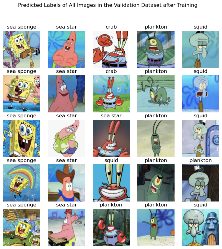
Again, we can see our model is working pretty well on the validation set.
Try it for yourself!
Can you make a better model than we made above? See if you can reduce the losses even further by implementing one of the following:
an additional convolutional layer
an additional linear layer
an additional dropout
variations in the augmentation
Key Takeaways
A convolutional neural network uses kernels with weights to learn key spatial patterns in a data set.
Convolutional neural networks are a common tool in image processing.
Dropout and data augmentation are two approaches to avoid overfitting in a neural network model.