Motivation
Machine learning is a popular topic these days, but in reality, it has been a topic of study for quite some time as a subset of data science. As a transition to thinking about machine learning approaches and algorithms, it’s helpful to consider a simple example common to data analysis - linear regression. In the subsequent subsections under Machine Learning Basics, we’ll use a set of linear regression examples to introduce machine learning terminology and a common framework that will apply to other algorithms and applications down the road. In this notebook, we’ll take a look at our example data - CO concentrations collected at the Mauna Loa Observatory a.k.a. the “Keeling Curve”.
Import modules
Begin by importing the modules to be used in this notebook:
import numpy as np
import matplotlib.pyplot as plt
import pandas as pd
Mauna Loa CO Measurements
For a concrete example, we will consider the trend in CO concentration in the atmosphere as measured at the Mauna Loa Observatory on the Mauna Loa volcano in Hilo Hawaii:
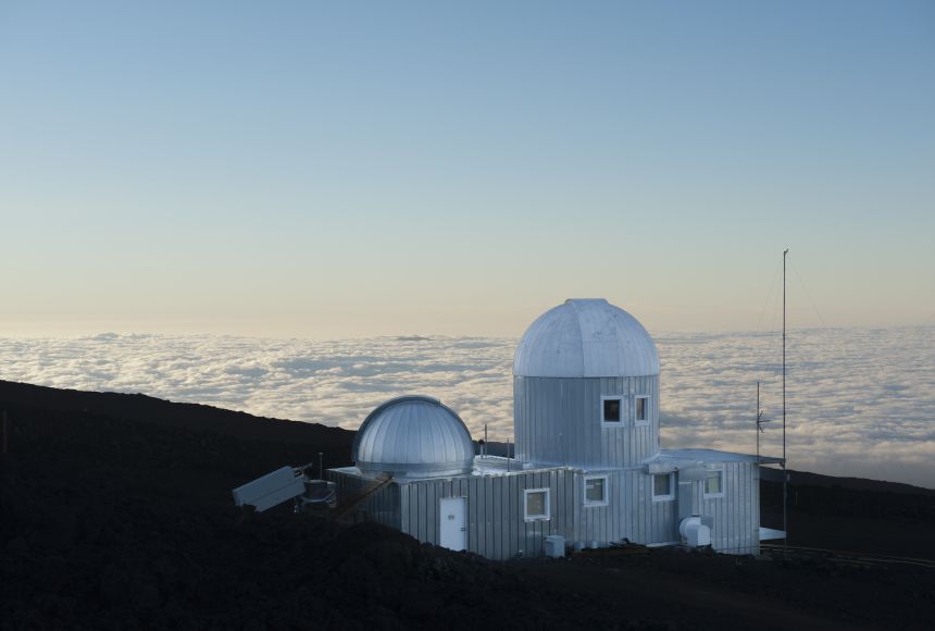
Photo Credit: Johnathon Kingston, National Geographic.
The record of CO concentrations collected at Mauna Loa, sometimes referred to as the “Keeling Curve” for its founding scientist, is a multi-decadal record that is available from the Scripps Institute of Oceanography HERE. The video HERE for information on how the data is collected.
Here, we will work the monthly data in this dataset, which is available in the monthly_in_situ_co2_mlo.csv file provided in the data directory of this book. Let’s read that in here:
# read in the dataset with pandas
df = pd.read_csv('../data/monthly_in_situ_co2_mlo.csv', skiprows=64)

# filter out null values stored as -99
df = df[df.iloc[:, 4] >0]

# the decimal year information is in the 4th column
x = df.iloc[:, 3]

# the CO2 information is in the 5th column
y = df.iloc[:, 4]
Let’s take a look at what this data looks like:
plt.figure(figsize=(8,4))
plt.plot(x,y,'k.')
plt.xlabel('x (year)')
plt.ylabel('y (CO$_2$ concentration, ppm)')
plt.show()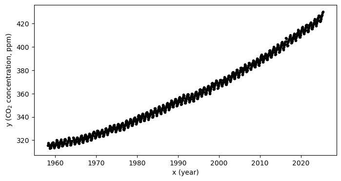
As we can see, this record extends back to the 1950’s and continues through present day. We’ll take a number of approaches to investigate this data in the next notebooks.